1. Introduction

The rainfall forecast modeling systems are available to monitor and warn flood and drought events in Thailand. There are two fundamental approaches which are dynamical and empirical methods for rainfall forecasting. The dynamical prediction is generated by physical model based on numerical analysis that represents the evolution in seasonal forecasting by using observed Sea Surface Temperature anomalies as a boundary condition. The empirical approach relies on the observed and measured data. It is used to analyse the atmospheric and oceanic variables in the real world [1].

Tropical rainfall is influenced strongly by nearby sea temperatures in the real world  [1]. Recently, there are some climate predictions used empirical relations between Sea Surface Temperature or SST and atmospheric variables [2]. The empirical approaches is the most widely used to predict the climate using linear regression, machine learning, artificial neural network, and the methods of data-driven handling [3, 4].

In this paper, the monthly rainfall forecasting model is implemented by using the convolutional autoencoder technique for efficient unsupervised encoding of image features. We used 7 years (2014-2020) datasets of the global climate data such as SST and the Global Satellite Mapping of Precipitation project or GSMaP datasets that both are the satellite images. This model has predicted the monthly rainfall amount in image format. This is the improvement of the data-driven analytics which is a project of Hydro – Informatics Institute (Public Organization) [5].

The monthly rainfall forecasting amount with 6 months ahead were predicted. The experimental results show the accuracy that was calculate between the prediction rainfall amount and the actual rainfall amount.

The remaining of this paper is organized as follows: Section 2 describes the background knowledge related to this work. Section 3 explains the analysis of SST matching. In section 4, the experimental results of monthly rainfall forecasting model are presented. Finally, this work is concluded in section 5.

2. Background

The datasets and image processing technologies using in this monthly rainfall forecasting model are described in this section.

2.1. Data

The set of data using in this work consist of two datasets that were SST as displayed in Figure 1 and the satellite precipitation or GSMaP as displayed in Figure 2. Firstly, SST is the ocean temperature that closes to the ocean’s surface. The sea surface is between 1 millimetre and 20 meters below the sea surface [6]. The weather satellite sensors are available to measure and define sea surface temperatures. Secondly, the GSMaP project [6,7,8,9] is a high resolution global precipitation map production applying satellite data. This project is supported by Core Research for Evolutional Science and Technology (CREST) of the Japan Science and Technology Agency (JST) during 2002-2007. The GSMaP project activities are promoted by the JAXA Precipitation Measuring Mission (PMM) Science Team since 2007.

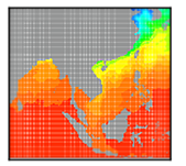Figure 1: The example of SST data.

Figure 2: The example of GSMaP data.

2.2. Type and Format of Data

Because SST and GSMaP are the satellite images in the digital formats, to display both on Map and to have a good performance, both are converted from images (JPEG) format to text (ESRI ASCII raster) format. The ESRI ASCII raster file format has the basic structure as illustrated in Table 1 [10]. The header fields at the top of the file displayed in “Parameter” column in Table 1 [10]. The example of ESRI ASCII raster file is shown in Figure 3.

Table 1: The description of the header fields of ESRI ASCII raster file.

Parameter	Description	Requirements
NCOLS	Number of cells in a column.	Integer
NROWS	Number of cells in a row.	Integer
XLLCENTER	Coordinate X on the origin point (at lower left corner of the cell).	Match with Y coordinate type.
YLLCENTER	Coordinate Y on the origin point (at lower left corner of the cell).	Match with X coordinate type.
CELLSIZE	Cell size.	Decimal
NODATA_VALUE	The value means NoData in the raster file.	Optional

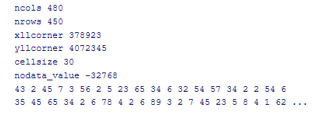Figure 3: The example of ESRI ASCII raster file.

2.3. Convolutional Autoencoder

A Convolutional Autoencoder or ConvAE shown in Figure 4 is a type of Convolutional Neural Network (CNN) designed for unsupervised deep learning. CNN is widely used in the field of pattern recognition. CNN architecture is constructed from various layers in the neural network. The convoluted layers are used for automatic extraction of an image feature hierarchy. The size of the input layer is the same as output layer. An autoencoder consists of image encoder and image decoder. The training of the autoencoder encodes image features into compressed images. The encoded image features are then clustered using k-means clustering. a small sub volume set is characterized by the decoded cluster center [11]. This technique is applied to reduce the storage usage, speeding up the computation time, improving performance by removing redundant variables [12].

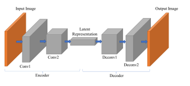Figure 4: Convolutional Autoencoder.

• An encoder as shown in Figure 4 is an algorithm used to transfer one format to another format. In this work, the encoder is applied to the original image. Then, the original image is represented in smaller feature vectors image or it is compressed [13].
• The decoder as shown in Figure 4 is an algorithm used for image decompression. The important features of the original image are not lost after the decoding process is applied in the encoded image. The compressed image is returned to its original image [13].

2.4. Image Retrieval

To retrieve the similar images stored in the images database and to get the top-k most similar database images, K-Nearest Neighbours or KNN method with cosine similarity as the distance metric. KNN is applied to verify the nearest neighbours and to get k nearest points as the similar images from a query image.

The Content Based Image Retrieval method was applied in this work as the process flow shown in Figure 5. In training process, the encoded representation of all images from training database is calculated using ConvAE and saved in a file. In testing process, the encoded representation of query image from testing database is calculated using ConvAE and saved in a file. The distance between the encoded representations of query image to encoded representation of all the images in training database is calculated to find nearest neighbors. Finally, KNN retrieves the top-k images in descending order of distance to the query image [14].

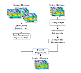Figure 5: The Content Based Image Retrieval process flow.

2.5. Image Matching

Image matching is method to evaluate the maximum similarity values between two digital images. The method is divided into two categories:  1) gray-based matching 2) feature- based matching. The gray-based matching is a matching algorithm of the grayscale feature applied in the image pixels. The feature-based matching is a matching algorithm of the feature vector points [15]. Image similarity is the similarity measurement between two images with the metrics. Therefore, some similarity criteria rules are used to verify the corresponding points of two images. The similarity quality is evaluated by the distance. Recently, there are many metrics of the distance measurement such as Euclidean distance, humming distance, cosine distance, and etc. the Hamming distance is a metric for measuring the distance between two binary strings.

2.6. Image Hashing

Image hashing has various methods which can be the mapping of the similar images with similar hashing codes. The well-known image hashing methods are the followings [16]:

• Average image hashing is the simplest hashing method. The images are converted to the greyscales which are transformed to binary codes with the average values.
• Perceptual image hashing extracts the real image features to hash values with discrete cosine transformation. This image hashing is the popular hashing method in signal processing.
• Difference image hashing uses the relative gradient technique to calculate the difference between adjacent pixels.

Hamming distance is the metric to compare and calculate the distance between two hashing strings. From comparing between the equal length of two hashing strings, hamming distance computes the number of bits which are different [17].

3. Sea Surface Temperature Matching

This section has described the convolutional autoencoder layers when the process was implemented and the image matching process for monthly rainfall forecast application.

3.1. Convolutional Autoencoder Layers

The convolutional autoencoder aims to predict monthly rainfall from the Sea Surface Temperature images. The rainfall predictor is implemented by adding the following layers to the neural network as described in Table 2 [13]. There is a procedure as the following:

• Step 1: A convoluted layer with shape of (287, 309, 16) is added and collected separately in the output layer 1. It is extracted significant features from the original image before reducing the shape in smaller features.
• Step 2: A maximum layer selected and pooled with the shape of (144, 155, 16), is associated to the first step convoluted layer and it resizes the layer to smaller features.
• Step 3: A dropout layer, with the shape of (144, 155, 8), is regularization technique to avoid overfitting of neural network.
• Step 4: A maximum layer pooled with the shape of (72, 78, 8), is associated to the previous step convoluted layer.
• Step 5: The previous maximum layer is pooled to the shape of (72, 78, 8) before a convoluted layer is applied.
• Step 6: A maximum layer selected and pooled with the shape of (36, 39, 8), is associated to the previous step convoluted layer.
• Step 7: The previous maximum layer is pooled to the shape of (36, 39, 8) before a convoluted layer is applied.
• Step 8: An upsampled layer with the shape of (72, 78, 8), is applied to increase the image resolution to the larger image shape.
• Step 9: The previous convoluted layer is performed by the additional operation on the output layer 2 with the shape of (72, 78, 8).
• Step 10: An upsampled layer with the shape of (144, 156, 8), is applied to increase the image resolution to the larger image shape.
• Step 11: The previous convoluted layer is performed by the additional operation on the output layer 1 with the shape of (142, 154, 16).
• Step 12: An upsampled layer with the shape of (284, 308, 16), is applied to increase the image resolution to the larger image shape.
• Step 13: The final layer of neural networks is applied to the convoluted layer with the shape of (284, 308, 4) to receive the output.

Table 2: The layers of Autoencoder method [13].

Layer (type)	Output Shape
Input Layer	(287, 309, 4)
Conv	(287, 309, 16)
Maximum Pooling	(144, 155, 16)
Conv	(144, 155, 8)
Maximum Pooling	(72, 78, 8)
Conv	(72, 78, 8)
Maximum Pooling	(36, 39, 8)
Conv	(36, 39, 8)
Upsampling	(72, 78, 8)
Conv	(72, 78, 8)
Upsampling	(144, 156, 8)
Conv	(142, 154, 16)
Upsampling	(284, 308, 16)
Conv	(284, 308, 4)

3.2. Image Retrieval Process

This application is the SST pattern data analysis for 6 months rainfall forecasting. In this work, the Content Based Images Retrieval technique to estimate the similarity values was applied in monthly rainfall forecasting of Thailand. Figure 6 illustrates the SST image matching process. The current SST has been detected and matched with the historical SST dataset stored in the database. In this project, MongoDB database application is used to collect the images which are the unstructured data. The program code is developed to retrieve the similar database images with comparing to the current SST images. The top three highest values of image similarities are the results of monthly rainfall forecasting.

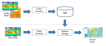Figure 6: The image matching process flow [5].

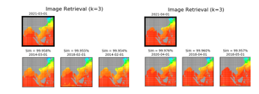Figure 7: The results of the top three highest SST similarities.

4. Experimental Results

The program has processed and generated the results of the top three highest SST similarities written by Python. These results are shown in Figure 7. The rainfall amounts using in this work are the accumulated rainfall or the accumulated GSMaP rainfall at the same months of top three highest SST matching. These months results are used to define the predicted months of rainfall data and they are shown on the application screen in Figure 8. In addition, the SST and GSMaP images can be simultaneously overlaid on application screen as illustrated in Figure 9.

The accurate measurement of this monthly rainfall forecasting analysis is described the detail of process in this section as well. The process flow is displayed in Figure 10. For this measurement, the image hashing method was applied to retrieve the GSMaP image similarities. The hashing codes are used to be the index to discover the most similar database images. The image hashing codes are used to compare the images which are easier and faster method than using the whole of original images [18].

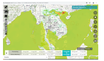Figure 8: The example of monthly GSMaP data overlaid on map.

Figure 9: SST and GSMaP data were overlaid simultaneously on the application screen.

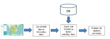Figure 10: The process flow of the accurate measurement of rainfall forecasting model [5].

The program code of accuracy evaluation of this monthly rainfall forecasting model by using image pattern similarity was written by Python Jupyter as shown in Figure 11. The current monthly GSMaP rainfall datasets were matched with the historical GSMaP datasets collected in MongoDB. Both of the current and the historical GSMaP hashing codes were created and then the similarity values between two images were computed with their hashing method. The example between the n^th months GSMaP rainfall forecasting and the n^th months of the historical matching GSMaP as shown in Table 3 and Table 4.

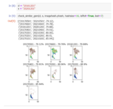Figure 11: The example of Python Jupyter displaying for GSMaP comparison.

Table 3: The example I of the rainfall forecasting date and the historical matching date of GSMaP data.

Forecasting date	History matching date
Dec. 2020	Dec. 2016
Jan. 2021	Jan. 2017
Feb. 2021	Feb. 2017
Mar. 2021	Mar. 2017
Apr. 2021	Apr. 2017
May 2021	May 2017
Jun. 2021	Jun. 2017

Table 4: The example II of the rainfall forecasting date and the historical matching date of GSMaP data.

Forecasting date	History matching date
Nov. 2020	Nov. 2016
Dec. 2020	Dec. 2016
Jan. 2021	Jan. 2017
Feb. 2021	Feb. 2017
Mar. 2021	Mar. 2017
Apr. 2021	Apr. 2017
May 2021	May 2017

The GSMaP rainfall images on the forecasting months were computed the similarity values with the historical GSMaP matching months. The example image of GSMaP similarity (%) case is shown in Figure 12.  In addition, the example of the similarity values of monthly GSMaP rainfall forecasting and their historical matching were calculated as shown in Table 5. Table 5 is the example 1 which shows the GSMaP data matching between forecasting months, 2020/12 – 2021/06, and history matching months, 2016/12 – 2017/06. The similarity values of example 1 are 81.21%, 93.18%, 84.14%, 83.75%, 82.3%, 79.53%, and 80.52%, respectively and the average of similarity values is 83.52%. For the example 2 in Table 6, the forecasting months are 2020/11 – 2021/05 that match with the history matching months, 2016/11 – 2017/05 and the similarity values are 81.46%, 81.21%, 93.18%, 84.14%, 83.75%, 82.3%, and 79.53%, respectively. The average of similarity values in the example 2 is 83.65%.

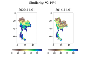Figure 12: The example images of GSMaP similarity (%)

Table 5: The example I of the average of monthly GSMaP forecasting and the historical matching similarity

Forecasting months	History matching months	Similarity (%)
2020/12	2016/12	81.21
2021/01	2017/01	93.18
2021/02	2017/02	84.14
2021/03	2017/03	83.75
2021/04	2017/04	82.3
2021/05	2017/05	79.53
2021/06	2017/06	80.52
	Avg.	83.52

Table 6: The example II of the average of monthly GSMaP forecasting and the historical matching similarity

Forecasting months	History matching months	Similarity (%)
2020/11	2016/11	81.46
2020/12	2016/12	81.21
2021/01	2017/01	93.18
2021/02	2017/02	84.14
2021/03	2017/03	83.75
2021/04	2017/04	82.3
2021/05	2017/05	79.53
	Avg.	83.65

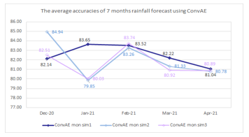Figure 13: The graph of the monthly rainfall forecast similarity since December 2020 to April 2021

Figure 13 is the comparison between the accurate values of top three highest similarities or top three rainfall forecasting. The graph shows the accurate values of 5 months GSMaP rainfall forecast since December 2020, January 2021, February 2021, March 2021, to April 2021.  The accurate values of the highest similarity (dark blue line) are 82.14%, 83.65%, 83.52%, 82.22%, and 81.04%, respectively. The average of the first accuracy is 82.51%. The average of the second and the third accurate values are 82.03% and 81.62%, respectively. Therefore, it can be found that the highest GSMaP rainfall forecast is better than others.

5. Conclusion

The monthly rainfall forecasting was the SST image patterns analysis by computing the average similarity between the recent monthly SST image datasets and historical monthly SST image datasets and applying convolutional autoencoder method to retrieve the top three highest of SST similarities. Moreover, the accurate value of this monthly rainfall forecasting was evaluated by applying the GSMaP image matching method as well. Then the result of this monthly rainfall forecasting was 82.514% which was an average value in matching GSMaP testing datasets.

However, this monthly rainfall forecasting model will be improved the accuracy, in the near future, by considering more atmospheric variables related to rainfall in Thailand. In addition, the weekly rainfall forecasting will be added in the application.

1. M. Kannan et al., “Rainfall Forecasting Using Data Mining Technique,” International Journal of Engineering and Technology, 2(6):397-401, 2010.
2. University of Reading, “Tropical Rainfall and Sea Surface Temperature Link Could Improves Forecast,” https://www.reading.ac.uk/news-and-events/releases/PR849878.aspx, 26 October 2020.
3. M. Haghbin et al., “Applications of soft computing models for predicting sea surface temperature: a comprehensive review and assessment,” Progress in Earth Planetary Science, 8:4, 2021, doi:10.1186/s40645-020-00400-9.
4. O. Ieremeiev, V. Lukin, K. Okarma, and K. Egiazarian, “Full-Reference Quality Metric Based on Neural Network to Assess the Visual Quality of Remote Sensing Images,” Remote Sensing, 12(15):2349, 2020, doi:10.3390/rs12152349.
5. P. Deeprasertkul, “An Assessment of Rainfall Forecast using Image Similarity Processing,” Proceedings of the 2020 3rd International Conference on Image and Graphics Processing, 141-145, 2020, doi:10.1145/3383812.3383821.
6. K. Okamoto et al., “The Global Satellite Mapping of Precipitation (GSMaP) project,” 25th IGARSS Proceedings, 3414-3416, 2005, doi: 10.1109/IGARSS.2005.1526575.
7. K. Aonashi, J. Awaka, M. Hirose, T. Kozu, T. Kubota, G. Liu, S. Shige, S. Kida, S. Seto, N. Takahashi, and Y. N. Takayabu, “GSMaP passive, microwave precipitation retrieval algorithm: Algorithm description and validation,” J. Meteor. Soc. Japan, 87A, 119-136, 2009.
8. T. Kubota, S. Shige, H. Hashizume, K. Aonashi, N. Takahashi, S. Seto, M. Hirose, Y. N. Takayabu, K. Nakagawa, K. Iwanami, T. Ushio, M. Kachi, and K. Okamoto, “Global Precipitation Map using Satelliteborne Microwave Radiometers by the GSMaP Project : Production and Validation,” IEEE MicroRad, 290-295, 2006, doi: 10.1109/MICRAD.2006.1677106.
9. T. Ushio, T. Kubota, S. Shige, K. Okamoto, K. Aonashi, T. Inoue, N. Takahashi, T. Iguchi, M. Kachi, R. Oki, T. Morimoto, and Z. Kawasaki, “A Kalman filter approach to the Global Satellite Mapping of Precipitation (GSMaP) from combined passive microwave and infrared radiometric data,” J. Meteor. Soc. Japan, 87A, 137-151, 2009, doi:10.2151/jmsj.87A.137.
10. ESRI Inc., “ESRI ASCII raster format,”
    http://resources.esri.com/help/9.3/arcgisengine/java/GPToolRef/spatial_analyst_tools/esri_ascii_raster_format.htm.
11. X. Zeng, M. Ricardo Leung, T. Zeev-Ben-Mordehai, and M. Xu, “A convolutional autoencoder approach for mining features in cellular electron cryo-tomograms and weakly supervised coarse segmentation,” Journal of Structural Biology, 202(2):150-160, 2018, doi:10.1016/j.jsb.2017.12.015.
12. Y. Zhang, “A Better Autoencoder for Image: Convolutional Autoencoder.” In ICONIP17-DCEC, 2018.
13. P. Kumar and N. Goel, “Image Resolution Enhancement Using Convolutional Autoencoders.” 7th Electronic Conference on Sensors and Applications Proceedings, 8259, 2020, doi:10.3390/ecsa-7-08259.
14. P. Deore, V. S. Patil, and V. B. Patil, “Content Based Image Retrieval using Deep Convolutional Variational Autoencoder,” Proteus Journal, 11 (10), 2020, ISSN/eISSN: 0889-6348.
15. G. Jianhua, Y. Fan, T. Hai, W. Jing-xue, and L. Zhiheng, “Image matching using structural similarity and geometric constraint approaches on remote sensing images,” Journal of Applied Remote Sensing, 10(4), 2016, doi:10.1117/1.JRS.10.045007.
16. T. Zhenjun, W. Shuozhong, Z. Xinpeng, and W. Weimin, “Structural Feature-Based Image Hashing and Similarity Metric for Tampering Detection,” Fundamenta Informticae, 106(1):75-91, 2011, doi:10.3233/FI-2011-377.
17. N. Raut, “What is Hamming Distance?,” TutorialPoint, 2018.
18. Study.com, “Discuss the advantages of hashing,” 2019.

(Click Here)