1. Introduction

This paper is an extension of work originally presented in conference Novel Intelligent and Leading Emerging Sciences Conference (NILES) [1]. As everybody knows that a human is intelligent and has an aural source separation that helps to identify singular sounds within a mixed sound. The type of mixed sound could be a speech or music, which can be detected via the human aural system; because the brain nerves are trained since birth to differentiate between human speech and music. Artificial intelligence, machine learning algorithms, and other Technological advancements have contributed to the revolution of machines to simulate the human intelligence.

Machine learning algorithms contributed to the development in multiple fields such as signal processing.  An approach called Blind Source Separation (BSS) can separate unknown set of source signals and the mixing methodology. Furthermore, BSS recovers all individual sources simultaneously as output from the mixture, which helps in performing a real-time technique.   Thus, BSS can process sounds in a real-time using many algorithms such as independent component analysis (ICA), Principal Component Analysis (PCA), Degenerate Unmixing Estimation Technique (DUET), Short Time Fourier Transform (STFT) [2], [3]. Some studies applied this methodology to improve other algorithms such as the Deep Neural Network (DNN) algorithm [4], the Independent Deeply Learned Matrix Analysis (IDLMA) algorithm [5], the Minimum-Volume Beta-Divergence (NMF) algorithm [6], and others.

The real-time approach can be applied simultaneously when using BSS. This enhances separation by using a synchronization procedure during processing. One of the most significant evaluation criteria for comparison is real-time processing because it prefers the algorithm that has a minimum execution time during the separation process.  The execution time value computes the actual time through the separation process.

This paper compares the efficiency of Conv-TasNet and Demucs algorithms which use the BSS approach to separate a mixture of two sounds (human speech and music). The biggest challenges are training and testing the algorithms to distinguish between original sounds with high-quality output signals in real-time, with a small execution time value.  Both algorithms implement a synchronization method, which substantially reduces the execution time and applies a multi-channel input audio source as well.

2. Related Work

In [7], the authors applied time-domain methodology with the BSS approach. They presented a real-time approach using a Deep Learning System (DLS), which is a robust speech processing during multi-talker environments. Moreover, the authors used signals on nonnegative encoder outputs through the encoder-decoder framework that implemented a model called Time-domain Audio separation Network (TasNet) [8]. The Wall Street Journal (WSJ0-mix) dataset was used to study speech separation problems using two speakers. The dataset was separated into testing and training sets randomly produced mixture. The evaluation appeared that the DLS was 0.23 milliseconds which is six times faster than the state-of-art based system [9]. Nevertheless, the DLS system is not applicable in this study, because DLS supports a short latency like telecommunication applications and listening devices. Furthermore, the experiment is limited only on speech for robust speech processing environment, which represents different object in this study.

Another study implemented Degenerate Unmixing Estimation Technique (DUET) with the Levenberg-Marquardt algorithm for improving the synchronization and signal ratio [10]. This study aimed to build a new DUET with a real-time application while enhancing the quality of the separation process. They used the Bach10 audio dataset [11], which has ten excerpts of classical music, and the single tracks are obtainable. The random mixing with distinct parameters was used to compute the simulated stereophonic mixtures. Using Signal-to-Interference Ratio (SIR), according to the evaluation, a higher SIR means a higher separation of signals quality where they found that SIR was 0.06. Improving the disjoint orthogonality between prediction and observations sources using a recursive implementation in Levenberg-Marquardt algorithm. This result added value to our research study; in terms of enhancing the quality of separation of the BSS in real-time.

In [12], the authors proposed Time-Frequency (TF) method with BSS by estimating the quantity of TF masks and sources with a current spatial aliasing problem. They used DUET and Observation Vector Clustering (OVC). Also, they developed offline and online approach to deal with spatial aliasing. The online separation algorithm operated on gradient ascent and single frame basis. In addition, it optimized using on gradient ascent search with fixed known of the maximum quantity of sources N. The audio dataset was the (CHAINS corpus) story [13]; the authors chose the six-voice signals of the story. Their experiments were implemented simulating a cocktail party situation.  Higher distance-miking is the best for the separation performance. The online algorithm was able to track moving sources by estimating of a fixed known of the maximum quantity of sources. The authors mentioned that in mildly reverberant environments, both offline and online algorithms show a good separation performance. However, they do not mention the processing speed of online or offline algorithms.

BSS approaches can be implemented in real-time on hearing aid systems [14]. It is possible to extract and reproduce the target component from mixed binaural sounds using a pocket-size real-time BSS module. The author compared Single-Input Multiple-Output (SIMO) of ICA module with SIMO-of binary masking on convolutive mixtures of speech. Then, produce binaural sounds from the decomposition of mixed binaural sounds. Their experiment evaluated both objectively and subjectively, using 9 users (8 male and 1 female). The distance between the sound source and user was 1.5 m. Furthermore, the speech sample was limited to 9 s and the sampling frequency was 8 kHz. The performance of the modules was comparatively high because of ICA value estimation. Besides, noise reduction rating NRR proposed as a better method rather than conventional methods. However, the authors did not mention more details about their datasets.

In [15], the authors used DUET algorithm of BSS in their research study.  They proposed random number of sources while using only two mixtures.  Tracking mixing parameters via an online algorithm was applied in a Maximum Likelihood based gradient search method. They generated a mixture dataset using different noises and voices, and they recorded varying angles in echoic and anechoic rooms. Anechoic and echoic rooms of 1500 tested mixtures, anechoic and echoic were 15 dB and 5 dB respectively, of office mixtures. The evaluation environment was a 750 MHz laptop computer, which run more than five times faster than real-time. They noticed that the separation results improved as the angle difference increased. The dataset of authors is completely different from our paper.

The Support Vector Machine (SVM) algorithm is also the solution of BSS under-determined convolutive problem. A study in [16], the authors applied an audio signals sparsity property as an alternative to the independence or stationery of the sources’ expectation. Their test was based on the vocal of male and female. They recorded the audio set in a room using microphones with 0.2 seconds of reverberation time.  The rate of sampling was 16KHz, and an interval of recording was 28 seconds. The authors presented visualization of signals, but without including a consistent description. The use of the SVM algorithm proved that the BSS could be enhancing via classification using the sparsity property during the separation procedure.

In [17]. the authors proposed optimization approaches about (DUET) algorithm. They developed and implemented DUET for distant speech recognition engine.  The authors used two standard techniques for BSS real time: omni-directional microphones and soundcard at reverberation environments. Also, they had several speakers and noise sources, such as a TV. Their experiment focused on two human speakers in a room. They studied the Maximum Microphone Distance (MMD) and became MMD >1m or 2m, but this was a negative effect on the separation quality. However, there are some factors should be considered in a real-time approach when there are multiple sources of a streaming algorithm using position tracking, correlation, arbitrary statistics, condensed metrics.  In addition to peak classier processed in 0.55s of execution time and running audio was 9.7s through a single thread with a five-intel core processor. They applied a huge and complex operations to come up with the result. Those techniques will be useful for creating new algorithms which has BSS in a real-time.

On the other hand, in [18], the authors introduced a BSS in real-time oriented to voice separation. They used low-power technique of a processor and synchronized signal for enhancing a real-time methodology. they focused on a cocktail party problem. The sampling rate was 8KHz and the size of data was 16 bit/sample. The audio sets were music, drum, male voice, and more recorded in an audio studio with a professional equipment environment. The authors realized that the algorithm was unable to increase the separation performance using a real-time approach; because of the high quality of separation procedure which requires five times level up iteration. Thus, their research study would be helpful in medical aspects. On the other hand, this research could be implemented in many signals field, mainly when there is a need of a real-time separation.

Demucs implements through following the methodology of WAVE-U-NET algorithm with some disagreements. WAVE-U-NET focuses on manipulating the feature on different period intervals for resampling feature maps frequently. Furthermore, Demucs convert the mixture audio signal into individual original audio signals. Also, Demucs has a technique which is a transferred convolution, that it requires low cost of computation and low memory [19] [20]. Conv-TasNet is a state-of-the-art approach for the separation procedure of speech and music, which helps waveform domain to predict a mask and to improve the whole spectrogram. In [20], the authors speed up the Conv-TasNet during source separation to enhance the execution time which supports a real-time methodology [21].

This paper is an extension of work [1] to study the effectiveness of the Natural Language on the separation process of Demucs and Conv-TasNet algorithms. The experiments’ inputs were English, Arabic and Chinese Audioset. This is for studding the ability of the algorithm to separate speech from music blindly, without any previous known of the language type.

In [22], the authors presented the graph-clustering algorithm of Chinese Whispers. The evaluation of their research focused on Natural Language Processing (NLP) issues such as language separation, acquisition of word sense disambiguation, and syntactic word classes. This concludes to employee many graphs in NLP to optimize the separation.

In [23], the authors introduced continuous Arabic speech segmentation. They aimed to use high segmentation accuracies in Concatenative Speech Synthesis and Continuous Automatic Speech Recognition Systems. A tonal language such as Arabic has multiple allophonic phonemes; that will increase the segments computational cost. There are several factors such as ambiguous boundaries between phonemes and allophonic variations, makes recognition more challenging and affect the speech segmentation accuracy. FFT algorithm uses two main methodology frequency and time domains. The evaluation signals are recorded in a constricted environment. The audio sets were Ayat from Qur’an with a duration time 45s. Authors selected 10 audio speeches of 10 readers recorded with no interfering sounds such as noise. The samples file are 128 samples with mono- channel, bit rate 128kbps, type was .wav, audio format is PCM and audio sample size are 16-bit. In segmenting, they had a high segmentation result of intensity value and continuous signals. In the Arabic vowels, the process of the algorithm was accurate at segmentation. This research cannot be compared with the our study results because the differences in algorithms type and propose. The dataset of the experiment is a Small World graphs (SW-graph) [24]. PCW algorithm can process a huge number of graphs in a standard time, however its nondeterministic produces indecisive results.

3. Research Methodology

In this section, we focus on two algorithms for signal separation blindly on a real-time that were used in this research. These algorithms are the Demucs and Conv-TasNet algorithms to compare. The two algorithms are supported and updated in year 2020 by Alexandre Défossez. Moreover, both algorithms are efficient at computational cost and memory process. They are comparable; because they are based on state-of-the-art approaches [20], However, they have an MIT license that can be used and edited. Both Conv-TasNet and Demucs employ machine-learning algorithms to build the models. Also, discuss the evaluation method via the performance of the algorithm and the input and output signals. This research study was extended [1] to apply the Natural Language (NL) of three different languages English, Arabic and Chinese.

TasNet time-domain audio separation network reproduced with the convolution evaluation and encoder-decoder convolutional architecture to come up with Conv-TasNet. The encoder-decoder architecture is like an ICA algorithm operation.  The input-signals of the algorithm are mixed sound. The encoder builds a convolutional block with a particular kernel amount. In addition, the output-signals are a decoders’ parameter produced in a non-negativity constraint form. Thus, the computational cost has a significant effect using long short-term memory (LSTM) network in the separation module process.  This produces a limitation while training the original TasNet algorithm; because of determining the shorter length of the segment’s waveform. Furthermore, LSTM requires a large quantity of parameters which has an immediate effect on expanding the cost of the operational procedure [21].

Conv-TasNet uses entirely time-domain convolution network for sound separation. It contains three stages of memory process: encoding, manipulating and decoding. At the first stage, the encoder module encodes the input signal into overlapping segments with a length (L). The selection depends upon the shorter L of a segment. The output of encoder becomes an input to the manipulating or separation stage, for estimating the mask of a waveform segments. The last stage is decoder, to transform the masks. It reverses the output of separation stage linearly to formulate the number of blocks. Figure 1 shows mathematically the Conv-TasNet process.

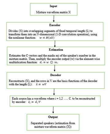Figure 1: The Stages of Conv-TasNet Algorithm

Conv-TasNet algorithm is the evolution of TasNet algorithm, with application of entirely time-domain convolution network. As shown in figure 1, with the addition of the Temporal Convolutional Network (TCN) methodology. TCN assists in reducing the complexity of the model and the capacity and also  reducing the computational cost. It can be applied with or without a real-time approach, minimize the execution time, and the precision of a separation process. In view of all these reasons, Conv-TasNet is suitable for our study. However, the algorithm has some limitation, it is incapable to denoise the signal or remove the artifacts of a signal such as reverberation or vibrations.  Nevertheless, using a multi-channel could solve this problem. Additional limitation is that the constant temporal length can failure with lengthy tracking.  Accordingly, this algorithm needs to develop in many aspects, such as accuracy and execution time.

Basic approach of Conv-TasNet algorithm is (1-D convolution separation model):

Algorithm Notation:

Y: is the input matrix

K: is the convolution kernel

P: is the kernel size

?_, and ?: are the rows on matrix Y and K, respectively.

L: is the convolution kernel with size 1.

⊛: is the convolution operation.

D-conv(.): each row of the input Y convolves with the corresponding row of matrix K.

S-conv(.): standard convolution which is a separable convolution.

Figure 2 clarify how the separation process of Conv-TasNet algorithm is in signals form. It shows the separation results on a signal form of Conv-TasNet of (Music &Female) category

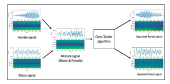Figure 2: Conv-TasNet Algorithm

On the other hand, Demucs algorithm applies the convolution models, which are encoders, decoders, and LSTM models.  Demucs is based on a U-network structure which is identical to the Wave-U-Net structure with differences. However, U-network performs a skip connection between the models, encoder, and decoder to supply a straight connection to the initial signal.  Although, U-network does not use linear interpolation but uses a transposed convolution. That helps reducing computational cost and the size of the memory, which enhances the utilization of memory and process four times less in general. Nevertheless, running out of memory is the limitation of the Demucs multi-channel. Figure 3 shows the Demucs process.

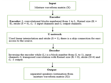Figure 3: Demucs Stages

There is discrepancy between Conv-TasNet and Demucs.  Demucs has a powerful decoder, that increments the kernel size 1 to 3, and the capacity as shown in table 1. Which gives advantage of preserve the lost information while mixing the instruments and unable to retain from the masking. Consequently, the disadvantage of retain information is execution time; because of the subsequent operations which could happen. Ultimately, time-domain and accuracy needs development.

3.1. Demucs General Equation

Basic approach of Demucs algorithm is (U-network structure), it uses Loss function to skip the association between encoder and decoder blocks to get straight transform to the initial input signal phase.

Algorithm Notation:

Figure 4 clarify how the separation process of Demucs algorithm is in signals form. shows the separation results on a signal form of Demucs of (Music &Female) category.

Table 1 shows the comparison between both algorithms depend on four features. These features are channel, kernel, time-domain, and speed.

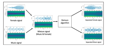Figure 4: Demucs Algorithm

Table 1: Conv-TasNet & Demucs Coperasion

Features	Conv-TasNet	Demucs
channel	2 multiple channels	(2 or more) Multiple channels
kernel	(K = 1) low capacity	Bigger capacity kernel size (K = 3)
time-domain	offline/online	offline/online
speed	high speed	low speed

The comparison is based on some measurements. First, the SciPy Python library has been used to compute the standard deviation (SD) for the reference source (mixture matrix) and the estimation source (separated matrix). Additionally, the signal-to-noise-ratio (SNR) is a measurement tool used to measure the noise ratio of the signals. Second, the Scikit Learn Python library has been used to calculate the coefficient of determination for constant input arrays instead of accuracy. Moreover, , there is a root mean square error (RMSE) which is a management tool used to measure the difference between predicted and actual values. The mean absolute error tool (MAE) has been used to measure the prediction error for the testing and training datasets. Finally, the actual execution time has been calculated using the Python Time package.  Since, this study is based on the BSS approach, it uses a performance evaluation package (mir_eval). It includes evaluation functions for music or audio signals. It has 4 measurement tools: (1) Signal-to-distortion-Ratio (SDR): it computes how is the similarity between the original signal and the produced signals, (2) Signal-to-Artifacts-Ratio (SAR): using artefacts helps in differentiate between the assessment errors, (3) Signal-to-Interference-Ratio (SIR) is the best measure of Gaussian noise and (4) Spatial-Distortion-Ratio (ISR) is A measurement tool usually used in image signals not in audio signal processing field.

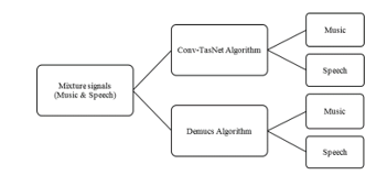Figure 5: Data Processing for two algorithms

The mixture sound signal could be a mix of Drum, Vocals, Bass, and others. Demucs and Conv-TasNet can be tested on this mixture to get the estimation sound signal. The objective of this research is to study two estimated sources: music and vocals. Thus, the methodologies of these algorithms have changed to conform to the needs, as shown in figure 5. Then, the file of input and output stored the quantitative data as digital metrics at txt file. The digital metric files reduce the execution time and memory process; because they reduce the cost to process digital NumPy array rather than the audio signal.

4. Dataset and Pre-Processing

The dataset in this research project was obtained from youtube.com to compare and evaluate the Demucs and Conv-TasNet algorithms [25].  The data contained in a file with a WAV format. The dataset grouped within five classification experiments: Music with Male, Female, Child, and Conversation. The total size of experiment files is 10GB which contains a duration time of each experiment. The duration time is 3 hours, 28 minutes, and 20 seconds equal to 2GB for every single group. Data selection depends on the negativity of noise ratio, the clarity, and the suitability for instance, pure classic music such as Jazz, Piano, and more. Moreover, pure male sounds such as speech in international conferences like TED talk AND Apple. These sounds have no background noise or interfering sounds. They are a continuous speech extracted from Youtube.com.  The factors (SD, SNR) of the pre-processing data were applied on all three languages mentioned before.

4.1. Data Types and signals

• Music (e.g., classical, piano, jazz): Figure 6 shows the jazz music acoustic vibrations.

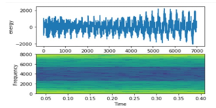Figure 6: Music Signal on top energy on bottom frequency

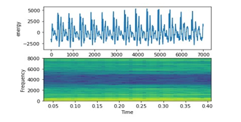Figure 7: English Female Signal on top energy on bottom frequency

• Female (e.g. Michelle Obama speech): Figure 7 shows a high frequency of female signal like seasonal indices.
• Female (e.g., Balqees Fathi speech in women power conference): Figure 8 shows a high English female frequency of signal like seasonal but sequence indices.

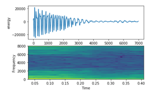Figure 8: Arabic Female Signal on top energy on bottom frequency

• Chinese Female Figure 9 shows a mid-frequency of signal comparing with other signals.

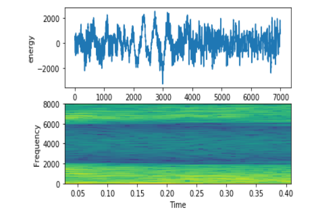Figure 9: Chinese Female Signal on top energy on bottom frequency

• Male (e.g., male speech from Apple conference): Figure 10 shows a low frequency of male signal. Males’ voices have lower intensity than females’ voices. This figure shows acoustic vibrations likes a screaming sound.

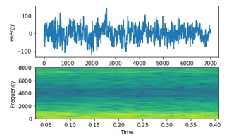Figure 10: English Male Signal on top energy on bottom frequency

• Male (e.g., male speech from TEDX speech): Figure 11 shows the lowest frequency of male signal. Males’ voices. This figure shows acoustic vibrations likes a screaming sound.

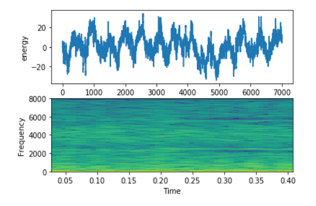Figure 11: Arabic Male Signal on top energy on bottom frequency

• Chinese Male: Figure 12 shows the highest frequency of male signal. Males’ voices. This figure shows more organized vibrations likes a seasonal.

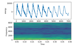Figure 12: Chinese Male Signal on top energy on bottom frequency

• Conversation (e.g., male and female discussion): Figure 13 shows a mix between male and female voices. The first part is a male vocal while the other part is a female vocal.

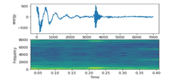Figure 13: English Conversation Signal on top energy on bottom frequency

• Conversation (e.g., male and female discussion): Figure 14 shows a mix between male and female voices. The first part is a male vocal while the other part is a female vocal. It looks unorganized signal.
• Conversation (e.g., male and female discussion): Figure 15 shows a mix between male and female voices. The first part is a male vocal while the other part is a female vocal. It looks unorganized signal.

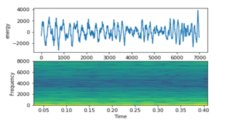Figure 14: Arabic Conversation Signal on top energy on bottom frequency

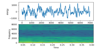Figure 15: Chinese Conversation Signal on top energy on bottom frequency

• Child (e.g., child stories): Figure 16 shows a high vibration at the beginning, but slightly decreasing at the end.

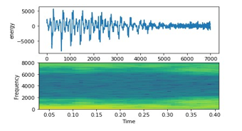Figure 16: English Child Signal on top energy on bottom frequency

• Child (e.g., child stories): Figure 17 shows a high frequency.

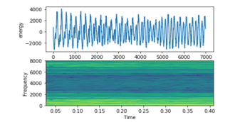Figure 17: Arabic Child Signal on top energy on bottom frequency

• Child (e.g., child stories): Figure 18 shows a high frequency and heigh vibration

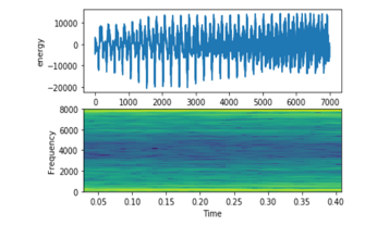Figure 18: Chinese Child Signal on top energy on bottom frequency

4.2. Data pre-processing

Jupyter and Python libraries have helped produce the input segments of the separation process by a pre-processing, which contains two operations split and merge. The first operation is splitting, which splits the 3 hours audio file of each category into 1250 segments. The second operation is merging, which merges 1250 Music segments with each category one by one. Figure 19 shows the steps of pre-processing data segments. The mixture segment resources have 10 seconds of duration time per segment. Each file consists of two original segment resources (music & male), (music & female), (music & child) or/and (music & conversation).

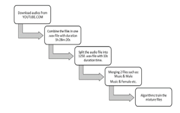Figure 19: Steps of pre-processing data

The experiments are based on six dataset files. The main file is an Excel sheet contains four columns: Youtube URL (object), start time (float), end time (float), and label (object). There are five files for each category, one of them is a music file contains 1250 Records with IDs and music names [26]. Moreover, Male, Female, Child, and Conversation have files with IDs and their names. This research study evaluated an audio dataset of ten gigabytes. each category had two gigabytes of mixture segments with a music dataset. In addition, these files related to the original files by IDs.  For each category of the dataset 70% was used for training and 30% for testing.  Numpy is a Python library used for randomizing splitting by randomize function. The experiment started with training data and then testing data of each mixture dataset.  Finally, measurement tools were used to evaluate the separation results.

4.3. Audio signals description in terms of SD and SNR

Standard Deviation (SD) is a measurement tool used to compute the data spreads (distribution) via computing the mean of squared deviations, then square root of the result. [25].

Table 2: The mean of standard deviation of all data

Mean	Music	Male	Female	Child	Conversation
English	0.111309	0.052772335	0.0523693	0.078172052	0.0620758
Arabic	0.111309	0.046679	0.022318	0.232547	0.083778
Chinese	0.111309	0.103396	0.107852	0.134417	0.086935

In table 2, the value of all columns = 0.1 SD. The results are closing to zero value, which indicates all the estimation values are near to the mean.

Signal-Noise-Ratio (SNR): is a measuring tool that calculates the ratio between the original signal with the artifact signal such as a noise. It computes the mean of a signal, then dividing the result by the SD [27], [28].

SNR = SD(MEAN(X))

Table 3: Signal-Noise-Ratio

Mean	Music	Male	Female	Child	Conversation
English	0.000257	-2.16667E-06	-4.53405E-6	-9.37E-06	-9.2014E-06
Arabic	0.000257	-3.80E-05	-9.94E-05	0.000168	-3.26E-05
Chinese	0.000257	0.000142	7.59E-06	-9.47E-05	0.000594

Table 3 shows the noise ratio of all categories. All SNR values are negative; this signifies a minimum noise ratio and considers as a pure signal. The negativity of SNR indicates as a high-quality score.

5. Experiments and Results

The audio datasets run on personal computer OMEN hp, i7 Intel core and 16GB of RAM. Using Python language for data processing via Jupyter and Pycharm. Using multiple packages such as: mir_eval Version: 0.5, Sklearn Version: 0.0, Scipy Version: 1.4.1, Pandas Version: 0.25.1, NumPy Version: 1.18.2, youtube_dl Version: 2020.3.24, Pydub Version: 0.23.1 and more. The audio files downloaded from Youtube.com via youtube_dl libraries. This downloading process took more than 2 hours per label. Merging Music files with all labels such as Male files via Overlay function this process takes 1 hour per label. After that, applying the data on Conv-TasNet and Demucs algorithms. For Demucs the process takes 6 hours and for Conv-TasNet the process takes 3 hours per label. The output of each algorithm produced 12.3 GB augments on the memory process, 1250 folders composed of 3750 files produced from each algorithm. Evaluation of each output for each algorithm takes 2 hours. this calculation for each 1250 WAV mixture files. Four experiments were applied for training and testing datasets, to study the effectiveness or speech classification for comparing the algorithms.  Four different data types were used in these algorithms: (Music & Male), (Music & Female), (Music & Conversation) and (Music & Child).

5.1. Evaluation Results

The comparison between Conv-TasNet and Demucs algorithms was based on seven measurement tools using three packages Scikit-Learn, mir_eval and time. Scikit-learn package supports three accuracy metrics: Mean Absolute Error (MAE), Root Mean Square Error (RMSE), and R square (R2).  Mir_eval package affords four tools to evaluate the performance: Spatial-Distortion-Ratio (ISR), Signal-to-Artefacts-Ratio (SAR), Signal-to-Interference-Ratio (SIR), and Signal-to-distortion-Ratio (SDR). Ultimately, the time package was used to calculate the execution time of the separation process.

The three tools were implemented to calculate the accuracy of the Conv-TasNet and Demucs algorithms. They support the quality score evaluation pertaining for observation inputs and estimation outputs. The observations cannot be calculated directly with accuracy because continuous metrics cannot apply to accuracy tools. RMSE, R2 and MAE were used to describe the results of algorithms.

• R Square (?^?)

It is a statistical tool used to measure the proportion of how close the data points to the fitted regression line. Via subtract the observed data with the data fitted on the line regression. In other words, it tells how data goodness fit the regression model [29] [30].

Training experiments:

Table 4: the experiments results pertaining to the (Music & Male and Music & Female) training dataset of all three languages.

Algorithm	Mean	Music & Male Experiment		Music & Female Experiment
		Music	Male	Music	Female
Demucs	English	0.594750505	0.554857091	0.652751885	0.706623375
	Arabic	0.906899	0.730184	0.817224	0.252617
	Chinese	0.911638	0.924542	0.890167	0.924055
Conv-TasNet	English	0.673642922	0.611274307	0.725606045	0.782790036
	Arabic	0.939895	0.913543	0.91162	0.155181
	Chinese	0.937934	0.936259	0.898883	0.925415

Table 4 shows that Music has an R-squared (?²) value of 59% and (Male) has an ?² value of 55%.  The ?² value can be more accurate if the noise ratio is low. For the ?² values described between 0% and 100%, 0% indicates that the observed data are far from the mean and have a low error estimation, while 100% indicates that the observed data are close to the mean [31].

As it shows that (Music & Male) experiments of both Arabic and Chinese are close to 100% which indicates the observed data are close to the mean. In another experiment, (Music & Female) of Arabic language is close to 0% which indicates the observed data are far from the mean and have a low error estimation.

Table 5: R Square of Conversation and child experiments of Training Dataset of all three languages.

Algorithm	Mean	Music & Conversation Experiment		Music & Child Experiment
		Music	Conversation	Music	Child
Demucs	English	0.641354444	0.682678489	0.624809687	0.763154352
	Arabic	0.938469	0.91497	0.67352	0.922591
	Chinese	0.865062	0.799423	0.884608	0.937521
Conv-TasNet	English	0.724467042	0.753158555	0.662892685	0.759285571
	Arabic	0.658099	0.000153	0.857881	1.16E-05
	Chinese	0.875329	0.822089	0.962708	0.477527

Tables 4 and 5 show the English language experiment results of Demucs algorithm, pertaining to the (Music & Female), (Music & Conversation) and (Music & Child) training datasets. The ?²               values of observation and prediction signals of each algorithm, are (Music) 65% and (Female) 70%, (Music) 64% and (Conversation) 68% and (Music) 62% and (Child) 76%, respectively. These results show that the (Music & Female) experiments achieved high ?² values and that (Child) also achieved a higher value of Demucs of training experiment. While (Music & Male) experiment of Demucs has the lowest value 59% and 55% respectively. On the other hand, Conv-TasNet achieved the highest value of ?², where (Female) ?² = 78%, that means Female signals are the most signals close to the mean. In this evaluation it is noticeable that the Conv-TasNet always has the higher value compared to Demucs. Demucs training experiment during Arabic language has the highest value of R square which is 93% at Music (Music & Male) experiment, while it has the lowest speech value 25% at Female (Music & Female) experiment. On another side, Conv-TasNet experiment during Chinese language has the highest value 96% at Music (Music & Child) experiment and Arabic language has lowest value at speech 0.0001% at (Music & Conversation) and (Music & Child) experiments.

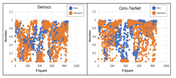Figure 20: ?²of (Music & Male) experiment of Demucs & Conv-TasNet of English language.

On another side, Arabic language with Demucs algorithm achieved the highest value of R-square at speech side (Male, Conversation and Child). Also, Chinese language usually has high value of R-square near to 100% which means better performance, close to the mean and low estimation errors on signals.

The right plot in figure 20 represents the R square of observation and prediction data of (Music & Male) of Demucs. The left plot shows the spread points of observation and prediction data of (Music & Male) of Conv-TasNet of training data. The blue points show the music data and orange points show the males speech data. It explains the spread of data point of observation and prediction data. X-axis represent the R square values of (Music & Male) experiment. The sample data is not the reason for the increased ?² value because all the experiments used the same number of segments. However, ?² result may be an effect of the lower noise ratio of observation.

Testing experiments:

Like the training experiment, all values in tables 6 and 7 are above 50%. The highest value of ?² is 77% of Conv-TasNet pertaining to the (Female) experiment and 67% of (Female) of Demucs algorithm.  In training and testing data experiments, training data has the same ?² with testing data which inference that data size sample has no affection of ?² value.

Table 6: ?² of male and female experiments of testing dataset

Algorithm	Mean	Music & Male Experiment		Music & Female Experiment
		Music	Male	Music	Female
Demucs	English	0.598482775	0.527509406	0.651269443	0.672236996
	Arabic	0.929927	0.90909	0.872887	0.54528
	Chinese	0.917021	0.908275	0.888142	0.911523
Conv-TasNet	English	0.677168022	0.659364504	0.712894379	0.774478377
	Arabic	0.927393	0.796538	0.958407	0.882355
	Chinese	0.966593	0.479971	0.85849	0.885474

Table 7: ?² of Conversation and Child experiments of Testing Dataset

Algorithm	Mean	Music & Conversation Experiment		Music & Child Experiment
		Music	Conversation	Music	Child
Demucs	English	0.645854253	0.681211663	0.624127646	0.756858895
	Arabic	0.8902	0.866712	0.744405	0.669279
	Chinese	0.865062	0.799423	0.893974	0.94875
Conv-TasNet	English	0.718706834	0.767224614	0.670057154	0.75645193
	Arabic	0.899566	8.36E-06	0.676389	0.000152
	Chinese	0.510896	0.393926	0.812849	0.910011

Demucs testing experiment during Arabic language has the highest value of R square which is 93% at Music (Music & Male) experiment, while English language has the lowest speech value 53% at speech (Music & Male) experiment. Also, at Arabic language with the value of speech 54% at (Music & Female) experiment. On another side, Conv-TasNet experiment during Chinese language has highest value 97% at Music (Music & Male) experiment; and Arabic language has lowest value at speech 0.000008% at (Music & Conversation) experiment and 0.0001 at (Music & Child) experiment.

        b- Root Mean Square Error (RMSE)

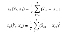
where ?² is the relative measure of the fit of the model, RMSE is the absolute measure of the fit. It is also a tool to measure how accurately the algorithm predicts the response. It can be used instead of accuracy tools because the accuracy tool does not support the continuous array of reference resources [32] [33].

Training experiments:

Tables 8 and 9 show the RMSE values for the (Music & Male), (Music & Female), (Music & Conversation) and (Music & Child) training datasets. The RMSE values are (Music) 0.06 and (Male) 0.04, (Music) 0.06 and (Female) 0.03, (Music) 0.06 and (Conversation) 0.03 and (Music) 0.06 and (Child) 0.03, respectively of Demucs. Lower values of RMSE indicate absolute fit. Overall, both algorithms have positive values from (0.3 to 0.6) which means that the observations and prediction data are close.

Arabic and Chinese language have lower value relatively with English language. Mostly, the value of RMSE is around 0.3 which indicates the absolute fit of the output signals comparing with English separation of both algorithms.

Table 8: Root Mean Square Error of Male and Female experiments

Algorithm	Mean	Music & Male Experiment		Music & Female Experiment
		Music	Mal	Music	Female
Demucs	English	0.060387951	0.035588642	0.055773658	0.026737967
	Arabic	0.028117	0.028008	0.039305	0.031757
	Chinese	0.030426	0.028518	0.034205	0.029987
Conv-TasNet	English	0.052309023	0.031107757	0.048070573	0.021558262
	Arabic	0.021331	0.021132	0.025871	0.025568
	Chinese	0.026394	0.025694	0.031611	0.030064

Table 9:  Root Mean Square Error of conversation and child experiments.

Algorithm	Mean	Music & Conversation Experiment		Music & Child Experiment
		Music	Conversation	Music	Child
Demucs	English	0.058033883	0.027021274	0.057891011	0.032158433
	Arabic	0.027798	0.024634	0.062237	0.064626
	Chinese	0.039827	0.038917	0.036068	0.033564
Conv-TasNet	English	0.04975772	0.020641371	0.053277448	0.032526892
	Arabic	0.061912	0.247073	0.042143	0.173703
	Chinese	0.033942	0.036129	0.019014	0.015994

 

Testing experiments:

Tables 10 and 11 show the RMSE values for the (Music & Male), (Music & Female), (Music & Conversation) and (Music & Child) testing datasets. Similarly, with training dataset, the values of Conv-TasNet and Demucs are almost the same. Overall, both algorithms have positive values from (0.3 to 0.6) which indicates that observations and prediction data are almost fit.

Like training data, the testing experiment also shows better results of RMSE of both languages Arabic and Chinese.

Table 10:  Root Mean Square Error of Male and Female experiments

Algorithm	Mean	Music & Male Experiment		Music & Female Experiment
		Music	Male	Music	Female
Demucs	English	0.061387858	0.038965244	0.058082848	0.02998228
	Arabic	0.024837	0.018296	0.03204	0.031994
	Chinese	0.024996	0.027324	0.034895	0.029049
Conv-TasNet	English	0.052586705	0.029218817	0.05128763	0.020946208
	Arabic	0.023592	0.023737	0.01534	0.014384
	Chinese	0.017425	0.013958	0.032243	0.031023

Table 11: Root Mean Square Error of conversation and child experiments.

Algorithm	Mean	Music & Conversation Experiment		Music & Child Experiment
		Music	Conversation	Music	Child
Demucs	English	0.05703156	0.026870191	0.059313099	0.032708388
	Arabic	0.033467	0.03027	0.041961	0.047127
	Chinese	0.039827	0.038917	0.030169	0.029733
Conv-TasNet	English	0.049186272	0.021074537	0.0546344	0.033307789
	Arabic	0.029296	0.156674	0.054295	0.24063
	Chinese	0.071935	0.080743	0.040955	0.040211

c- Mean Absolute Error (MAE)

MAE is a tool for measuring the accuracy of training algorithms. It handles continuous NumPy arrays and can be used to enhance the results of RMSE when measuring the algorithms’ predictions. It computes the average magnitude of the errors that occur between predictions and actual observations.

Training experiments:

Notably, tables 12 and 13 show (Female) and (conversation) of training dataset experiments, via Conv-TasNet get the smallest value of error 0.01 between the reference and estimation resources. Demucs has 0.04 of (Music) of all experiments and 0.02 of each speech (Male, Female, Conversation and child).

Table 12: Mean Absolute Error of male and female experiments.

Algorithm	Mean	Music & Male Experiment		Music & Female Experiment
		Music	Male	Music	Female
Demucs	English	0.043319834	0.023187058	0.039918792	0.016335086
	Arabic	0.015769	0.015549	0.02708	0.022367
	Chinese	0.018334	0.016945	0.021714	0.019184
Conv-TasNet	English	0.036686502	0.020443172	0.034022512	0.01306448
	Arabic	0.012075	0.011286	0.015174	0.014449
	Chinese	0.016413	0.015721	0.019738	0.018671

Table 13: Mean Absolute Error of conversation and child experiments.

Algorithm	Mean	Music & Conversation Experiment		Music & Child Experiment
		Music	Conversation	Music	Child
Demucs	English	0.041430066	0.016731485	0.040630954	0.018055779
	Arabic	0.017914	0.015582	0.045522	0.047743
	Chinese	36.54131796	14.75716936	35.2270372	15.65436042
Conv-TasNet	English	0.034715515	0.012663916	0.035056178	0.016750811
	Arabic	0.045405	0.18224	0.029647	0.121688
	Chinese	30.34135987	11.05559904	0.012242	0.010555

Notably Demucs algorithm at training experiment shows the highest performance of Music separation 0.02 MAE in Arabic language of both (Music & Male) and (Music & Conversation) experiments as well as Chinese language at (Music & Male) experiment. Chinese language has significant values – highest value of error – through (Music & Conversation) and (Music & Child) experiments, these values are (36.5 & 14.8) and (35.2 & 15.7), respectively.  Additionally, Conv-TasNet algorithm in training experiment shows the highest performance of Music separation 0.01 MAE in Arabic language at (Music & Male) experiment. However, Chinese language has significant values (30.3 & 11.1) at (Music & Conversation) sequentially which considered as the lowest performance in separation process.

Testing experiments:

Comparably, tables 14 and 15 of testing dataset experiment are like training dataset experiment of MAE values.

Table 14: Mean Absolute Error of male and female experiments.

Algorithm	Mean	Music & Male Experiment		Music & Female Experiment
		Music	Male	Music	Female
Demucs	English	0.044283635	0.025880494	0.041179648	0.018042131
	Arabic	0.013289	0.009229	0.020964	0.020834
	Chinese	0.015598	0.016635	15.89534399	6.964262591
Conv-TasNet	English	0.0370836	0.019214275	0.035862557	0.012616786
	Arabic	0.013402	0.013194	0.008488	0.007984
	Chinese	46.01418709	25.07100812	13.37673393	4.706061233

Table 15: Mean Absolute Error of Conversation and Child experiments

Algorithm	Mean	Music & Conversation Experiment		Music & Child Experiment
		Music	Conversation	Music	Child
Demucs	English	0.040552242	0.016646969	0.041642397	0.018309848
	Arabic	0.020308	0.017798	0.029497	0.033534
	Chinese	0.010246	0.007809	0.019657	0.019533
Conv-TasNet	English	0.034867332	0.013045045	0.036287197	0.017151002
	Arabic	0.019533	0.102707	0.038631	0.174129
	Chinese	0.056936	0.064269	0.024952	0.024837

In Demucs testing experiment, Arabic language has 0.01 at Music (Music & Male) experiment.  Chinese language has 0.01 at Music (Music & Conversation) experiment. Nevertheless, Chinese language has highest value (15.9 & 6.10) at (Music & Female) experiment that indicates a high error rate through separation process. Conv-TasNet testing experiment has lowest error 0.01 in Chinese language at Music (Music & Conversation) experiment. On another side, Chinese language has a high error after separation process; the values are 46.0 & 25.1 at (Music & Male) experiment and 13.4 & 4.7 at (Music & Female) experiment.

5.2. Mir_eval of (SDR, SAR, SIR, ISR)

It is a Python package used to evaluate the results, which retravel machine learning algorithms.  It extracts the music separation information pertaining to reference and estimation resources. Mir_eval package quantitatively compares the signals to algorithm implementations. The original mir_eval is a bss_eval package, which has been developed to evaluate the audio and image signals [34].

Training experiments:

Table 16: mir_eval of male and female experiments

Algorithm	SDR	Music & Male Experiment		Music & Female Experiment
		Music	Male	Music	Female
Demucs	English	6.365845562	2.261560323	7.724350679	5.891797598
	Arabic	14.34474	4.531938	11.95328	-4.01775
	Chinese	12.42069	11.31496	12.1474	11.05148
Conv-TasNet	English	7.768486164	2.785485859	9.208170136	7.873549345
	Arabic	14.66376	11.28408	14.29149	-5.51784
	Chinese	13.49518	12.34095	12.57517	11.18431
SIR
Demucs	English	6.365845562	2.261560323	7.724350679	5.891797598
	Arabic	14.34474	4.531938	11.95328	-4.01775
	Chinese	12.42069	11.31496	12.1474	11.05148
Conv-TasNet	English	7.768486164	2.785485859	9.208170136	7.873549345
	Arabic	14.66376	11.28408	14.29149	-5.51784
	Chinese	13.49518	12.34095	12.57517	11.18431

SDR is the signal distortion ratio.  It describes how similar the estimation resources are to the reference resources. SDR provides a global performance measure; but the other three measures are also important. Tables 16 and 17 show the average SDR values, taken from all the tracks.  In these tables, Conv-TasNet produces a higher SDR score for the (Female & Music) experiment, and for the (Child) training data set where (Child) = 8.3 SDR’. In turn, Conv-TasNet produces a lower SDR score for the (Child & Music) training data set where (Music) = 6.6 SDR for the (Music) training dataset and a smaller SDR value where (Male) = 2.8 SDR for the (Male & Music). On the other side, Demucs produces a higher value where (Music) = 7.7 SDR for the (Female) training dataset and where (Child) = 8.1 SDR for the (Music & Child) experiment. However, it produces a lower SDR score where (Music) = 6.4 SDR and 6.5 SDR, respectively, for the (Male) and (Child) training datasets and where (Male) = 2.3 SDR for the (Male) training dataset.

Comparing between the language experiments at Table 19, The highest SDR is in an Arabic experiment. Where Music values around 11 to 14 SDR and Male speech, but Female speech has the lowest value -4 and -5 SDR in both algorithms. While Chinese experiment has a heigh value 11 to 12 at Music and Male or Female speech.

Table17: mir_eval of conversation and child experiments

Algorithm	SDR	Music & Conversation Experiment		Music & Child Experiment
		Music	Conversation	Music	Child
Demucs	English	7.332337909	4.889571299	6.460674567	8.145132574
	Arabic	13.08034	10.58806	3.800309	11.54092
	Chinese	10.14399	6.673121	9.924395	12.20906
Conv-TasNet	English	8.941261981	7.486695151	6.626825047	8.292722159
	Arabic	3.972427	3.972427	8.91058	-26.6596
	Chinese	10.63976	7.20355	16.42239	-8.05199
SIR
Demucs	English	7.332337909	4.889571299	6.460674567	8.145132574
	Arabic	13.08034	10.58806	3.800309	11.54092
	Chinese	10.14399	6.673121	9.924395	12.20906
Conv-TasNet	English	8.941261981	7.486695151	6.626825047	8.292722159
	Arabic	3.972427	3.972427	8.91058	-26.6596
	Chinese	10.63976	7.20355	16.42239	-8.05199

At Table 17, there are more significant results of SDR affected by NL. Arabic experiment of Demucs algorithm has 13 at Music of conversation speech separation, but it has 3.8 SDR at Music of Child speech separation. On another side, Conv-TasNet algorithm during Arabic separation of conversation experiment is 4 SDR. While the lowest value in training experiment is -26.7 SDR.

Testing experiments:

One the other side, Conv-TastNet and Demucs have the higher values of (Child) testing dataset experiment, both values are 8.02 SDR. Then, (Conversation), (Female) and (Male) of testing dataset experiments respectively. SIR and SDR have the same values, which means a high correlation between these two measures.  This is further indicated by the fact that they dominated in terms of estimation error.  However, SIR is the best measure of Gaussian noise, while SDR focuses more on interference-level intrusiveness and separation [35]-[37].  The experiments in this research study illustrated that Conv-TasNet is a preferable algorithm from the perspective of SDR and SIR. The reason is Demucs using a larger window-frame size’.  Increasing weighting for noise power can cause potential modification of the SDR measure.

Table 18 and 19, in the context of comparing the Conv-TasNet algorithm with other research in terms of SDR, in [2], the authors have trained four models using the MusDB dataset [38], with 100 songs through Demucx, Conv-TasNet, Open-Unmix, MMDnseLSTM and Wave-U-Net. The average SDR of the vocals was 6.81 for the Conv-TasNet algorithm (the higher score) and 7.61 for the MMDnseLSTM algorithm. Their research study focused on music separation, while our research focused on music and speech separation in four categories.  The highest value of music SDR separation for the (Music) and Female datasets was in Conv-TasNet. Moreover, there are some classification experiments that produced scores even higher than those found in [9], such as the Child, Female and Conversation training datasets. For Demucs algorithm, the score of SDR was 8.15 in the Child dataset; this was higher than the reported in [9], (6.08 for MusDB and 7.08 for 150 extra song tracks).

Table 18: mir_eval of Male and Female experiments

Algorithm	SDR	Music & Male Experiment		Music & Female Experiment
		Music	Male	Music	Female
Demucs	English	6.303056998	1.461799732	7.607939697	4.703374514
	Arabic	12.92352	10.95636	11.55566	1.264586
	Chinese	11.78847	10.37697	10.47468	10.54035
Conv-TasNet	English	6.303056998	1.461799732	7.607939697	4.703374514
	Arabic	15.76899	6.375536	14.3024	9.198612
	Chinese	17.21237	-7.92302	9.808399	10.60297272
SIR
Demucs	English	6.303056998	1.461799732	7.607939697	4.703374514
	Arabic	12.92352	10.95636	11.55566	1.264586
	Chinese	11.78847	10.37697	10.47468	10.54035
ConvTasNet	English	6.303056998	1.461799732	7.607939697	4.703374514
	Arabic	15.76899	6.375536	14.3024	9.198612
	Chinese	17.21237	-7.92302	9.808399	10.60297272

Table 19: mir_eval of conversation and child experiments

Algorithm	SDR	Music & Conversation Experiment		Music & Child Experiment
		Music	Conversation	Music	Child
Demucs	English	7.390943771	4.908684372	6.583362429	8.02266854
	Arabic	11.81469	8.604822	6.909017	6.11558
	Chinese	10.14399	6.673121471	10.3703	13.03493
Conv-TasNet	English	8.912469304	7.531863904	6.66059257	8.02425869
	Arabic	10.93189	-26.1081	4.572872	-26.5985
	Chinese	1.261381	-0.95342	8.354678	10.88152
SIR
Demucs	English	7.390943771	4.908684372	6.583362429	8.02266854
	Arabic	11.81469	8.604822	6.909017	6.11558
	Chinese	10.14399	6.673121471	10.3703	13.03493
Conv-TasNet	English	8.912469304	7.531863904	6.66059257	8.02425869
	Arabic	10.93189	-26.1081	4.572872	-26.5985
	Chinese	1.261381	-0.95342	8.354678	10.88152

In [8], the author studied the application of the Conv-TasNet algorithm to the WSJ0-3mix dataset for speech separation. Their study focused on how causality for Conv-TasNet that is a causal configuration due to causal convolution and/or layer normalization operations, leads to drops in Conv-TasNet performance. The SDR of causal Conv-TasNet value is 8.2, while the corresponding value is 13.1 for non-causal Conv-TasNet. The high SDR score for non-causal Conv-TasNet refers to the high signal noise ratio that is equal to 12.7, while -0.00001 SNR of music tracks of this research.

Notably, the signal-to-artifacts ratio (SAR) value has no correlation to the SIR and SNR values because it calculates the quantization and interferences of signals. It assists in distinguishing between the estimation errors using artefacts. For all the experiments of different languages and algorithms, SAR has zeros value. Spatial-Distortion-Ratio (ISR) is more often used for image signal processing than audio signal processing. For all the experiments of different languages and algorithms, ISR has infinite value. The mir_eval package is limited when it comes to auditory signification. For instance, SIR can hardly distinguish between two different variables. In addition, SDR does not  compute the total perceived distortion in accurate manner.

5.3. Execution time

Figure 21 shows that Demucs separated (Music & Male) faster than (Conversation & Music), (Child & Music) and (Female & Music) of training and testing datasets respectively. Conv-TasNet separated (Female & Music) faster than (Music & Male), (Child & Music) and (Conversation & Music) in training dataset respectively.  A slightly different in ms is between (Child & Music) and (Conversation & Music), but (Conversation & Music) was faster than (Child & Music) in testing dataset. Also, figure 21, shows the average execution time in nanoseconds per track of Conv-TasNet that was seven times faster than Demucs, for testing and training datasets in all languages’ experiments. Conv-TasNet could be applied in real-time better than Demucs. Demucs needs further development, comparing with Conv-TasNet delay time. In [2], the author computed the speed of training of Demucs as 1.6 seconds and of Conv-TasNet as 0.7 seconds. However, this comparison is not accurate enough for consideration.  The reason is that the Conv-TasNet was applied to only two seconds of track duration; also, for Demucs using a different sample size significantly affected the actual processing time. Noticeable, that there was a slightly different in execution time between different natural languages around 0.1 which is not necessary to be mentioned, because the separation process of algorithms does not affect by NL. The results from each algorithm were based on some equations to perform a separation process.  The equations of each algorithm and their notations have mentioned before in research methodology section.

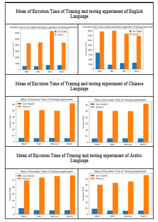Figure 21: The mean of execution time of English, Arabic and Chinese languages.

In general, after calculating the sum of execution time in nanoseconds (ns) of each separation process of languages. training and testing Demucs experiment, English is 202.3 ns and 203.2 ns the fastest at separation process, respectively. However, Arabic is 216.1 ns and 225.1 ns the slowest at separation process, respectively. Training and testing Conv-TasNet experiment, English is 29.1 ns and 29.4 ns the slowest at separation process, respectively. Nevertheless, Chinese is 23 ns faster than English and Arabic at Training experiment. While Arabic is 25.9 ns faster than English and Chinese at Testing experiment, See Appendix Table 20-25.

6. Conclusion

This research study compared the Conv-TasNet and Demucs algorithms. Both algorithms use BSS approach during the separation process. Conv-TasNet and Demucs estimate the number of blind sources to be separated into four sources: drums, bass, vocals and other. However, this research reduces the number of sources to be two, which are vocal and music. These algorithms are based on two approaches: real-time and blind-source separation. A random 10GB audio set was taken from Youtube.com.  These data separated into five categories: Male, female, Music, Conversation and Child. Using three Natural languages, which is English, Arabic and Chinese [25]. The performance with different and specific sources has been tested. The results show Conv-TasNet has excellent performance in separating music and speech sources. The highest SDR score of music is 9.21 in the female experiment, while the highest SDR score of speech at child experiment is 8.14. In addition, the average execution time of Conv-TasNet algorithm is seven times faster than Demucs algorithm.   With the NL extend, in general, Chinese language has high performance at source separation process during Demucs and Conv-TasNet algorithms in training and testing experiments. However, there are some significant values of separation performance at (Music & Conversation) experiment. The values are (15.9 & 6.10) indicate high MAE error.  Both algorithms have high error during source separation process of Chinese (Music & Conversation) experiments. The mixture signal contains Music and Male & Female Conversation.

Supplementarily, in general, Arabic language has high performance during Demucs separation process at (Music & Male). Normally, English language shows minor results comparing with Arabic and Chinese languages during both separation algorithms as it mentioned from table 6 to table 12.

There are some limitations in this research study.  Noise reduction was attempted with multiple algorithms such as (spectral gating of noise reduction [38], Deep Convolutional Neural Networks for Musical Source Separation [39], aasp-noise-red [40], Deep Audio Prior – Pytorch Implementation [41], Joint Audio Correction Kit (J.A.C.K.) [42] and more).  Nonetheless, those attempts were unsuccessful because the environment needs to be python 2. Old libraries are no longer supported for instance: J.A.C.K algorithm for noise reduction implemented on Python 3 via Pycharm. There was a lot of errors fixed by the researcher but after loading the input files there was no results because there is a runtime errors, which is one of the difficult errors to be tracked and fixed.  The Demucs algorithm could not support large amount of data. The dataset was 10GB, but the Demucs algorithm started to lose values without separating after training 8GB. The Authors have environment limitation to run Demucs GPU version, because it needs to be run on a wider range of hardware.

The future work of this research will focus on training more audio sets or different audio sets, using different algorithms like deep learning approach to separate the data and increasing the number of data categories. In addition, noise reduction can be a function inside the BSS algorithms.  The Conv-TasNet algorithm requires evolution in terms of actual time separation, computational cost and development of the separation process to achieve 100% interference separation. In addition, use the NL process functions in both algorithms could lead to a different and significant results.

1. A. Alghamdi, G. Healy, H. Abdelhafez “Real Time Blind Audio Source Separation Based on Machine Learning Algorithms”, IEEE 2nd Novel Intelligent and Leading Emerging Sciences Conference (NILES), 35-40, Oct, 2020, doi:10.1109/NILES50944.2020.9257891
2. M. Pal, R. Roy, J. Basu, M. S. Bepari, “Blind Source Separation: A Review and Analysis,” 2013 International Conference Oriental COCOSDA held jointly with 2013 Conference on Asian Spoken Language Research and Evaluation, 1-5, 2013, doi:10.1109/ICSDA.2013.6709849.
3. K. Ball, N. Bigdely-Shamlo, T. Mullen, K. Robbins, “PWC-ICA: A Method for Stationary Ordered Blind Source Separation with Application to EEG,” Computational intelligence and neuroscience 2016(73), 1-20, 2016, doi:10.1155/2016/9754813.
4. E. M. Grais, H. Wierstorf , D. Wa, R. Mason and M. D. Plumbley, “Referenceless Performance Evaluation of Audio Source Separation using Deep Neural Networks.,” 27th European Signal Processing Conference (EUSIPCO). IEEE, 1-5, 2019.
5. N. Makishima, S. Mogami, N. Takamune, D. Kitamura, H. Sumino, S. Takamichi , H. Saruwatari and . N. Ono, “Independent Deeply Learned Matrix Analysis for Determined Audio Source Separation,” EEE/ACM Transactions on Audio, Speech, and Language Processing, 27(10), 1601-1615, 2019.
6. V. Leplat, N. Gillis, M. Shun Ang, “Blind Audio Source Separation with Minimum-Volume Beta-Divergence NMF,” IEEE Transactions on Signal Processing, 68, 3400 – 3410, 2020, doi: 10.1109/TSP.2020.2991801.
7. Y. Luo and N. Mesgarani, “TASNET: TIME-DOMAIN AUDIO SEPARATION NETWORK FOR REALTIME, SINGLE-CHANNEL SPEECH SEPARATION,” IEEE/ACM Transactions on Audio, Speech, and Language Processing, 27(8), 1256-1266, 2019, doi: 10.1109/TASLP.2019.2915167.
8. G. Wichern, M. Flynn, J. Antognini, E. McQuinn, “WHAM!: Extending Speech Separation to Noisy Environments,” Sep. 2019. [Online]. Available: http://wham.whisper.ai/.
9. Lab Neural Acoustic Processing, “NEURAL ACOUSTIC PROCESSING LAB,” 2019. [Online]. Available: http://naplab.ee.columbia.edu/tasnet.html.
10. D. Fourer G. Peeters, “Fast and adaptive blind audio source separation using recursive Levenberg-Marquardt synchrosqueezing,” IEEE International Conference on Acoustics, Speech and Signal Processing (ICASSP), 766-770, 2018, doi: 10.1109/ICASSP.2018.8461406.
11. B. Pardo, “Interactive Audio Lab,” 2018. [Online]. Available: https://interactiveaudiolab.github.io/.
12. B. Loesch, B. Yang, “Blind source separation based on time-frequency sparseness in the presence of spatial aliasing,” International Conference on Latent Variable Analysis and Signal Separation. Springer, Berlin, Heidelberg, 1-8, 2010.
13. Informatics, UCD School of Computer Science and, “CHAINS characterizing Individual Speakers,” 2006. [Online]. Available: https://chains.ucd.ie/.
14. Y. Mori, T. Takatani, H. Saruwatari, K. Shikano, T. Hiekata, T. Morita, “High-presence hearing-aid system using DSP-based real-time blind source separation module.,” IEEE International Conference on Acoustics, Speech and Signal Processing-ICASSP’07, IV-609, 2007.
15. S. Rickard, R. Balan and J. Rosca, “Real-time time-frequency based blind source separation,” AJE, pp. 1-2, 2001.
16. H. Abouzid and O. Chakkor, “Blind source separation approach for audio signals based on support vector machine classification.,” Proceedings of the 2nd international conference on computing and wireless communication systems, pp. 1-6, 2017, doi: 10.1109/ICASSP.2007.366986.
17. A. Ferreira, D. Alarcão, “Real-time blind source separation system with applications to distant speech recognition.,” Applied Acoustics, 113, 170-184, 2016, doi: 10.1016/j.apacoust.2016.06.024.
18. D. J. Watts. Small Worlds: The Dynamics of Networks between Order and Randomness, Princeton Univ. Press, Princeton, USA, 1999.
19. D. Stoller, S. Ewert, S. Dixon, “Wave-U-Net: A Multi-Scale Neural Network for End-to-End Audio Source Separation,” 19th International Society for Music Information Retrieval Conference (ISMIR 2018), 334-340, 2018.
20. A. Défossez, U. Nicolas, B. Léon and B. Francis, “Music Source Separation in the Waveform Domain,” 1-16, 2019, arXiv preprint arXiv:1907.02404.
21. Y. Luo, N. Mesgarani, “Conv-TasNet: Surpassing Ideal Time-Frequency Magnitude Masking for Speech Separation,” IEEE/ACM transactions on audio, speech, and language processing 27(8), 1256-1266, 2019, doi: 10.1109/TASLP.2019.2915167.
22. C. Biemann “Chinese Whispers – an Efficient Graph Clustering Algorithm and its Application to Natural Language Processing Problems”, Workshop on TextGraphs New York City, 73–80, June 2006.
23. M. M. Awais; WaqasAhmad; S. Masud; S. Shamail, “Continuous Arabic Speech Segmentation using FFT Spectrogram”, Innovations in Information Technology conference, 2006, doi: 10.1109/INNOVATIONS.2006.301939.
24. D. Pani, A. Pani, L. Raffo, “Real-time blind audio source separation: performance assessment on an advanced digital signal processor,” The Journal of Supercomputing 70 (3), 1555-1576, 2014, doi:10.1007/s11227-014-1252-4.
25. Arwa-Data-Analytics, Machine-Learning-Algorithms-for-Real-Time-Blind-Audio-Source-Separation-with-Natural-Language-Detect, Retrieved from GitHub: https://github.com/ArwaDataAnalytics/Machine-Learning-Algorithms-for-Real-Time-Blind-Audio-Source-Separation-with-Natural-Language-Detect, July 23, 2021.
26. “scipy.org,” ENTHOUGHT, 26 Jul 2019. [Online]. Available: https://docs.scipy.org/doc/numpy/reference/generated/numpy.std.html. [Accessed 12 April 2019].
27. W. Gragido, J. Pirc, D. Molina, Blackhatonomics, Science Direct .com, 2013.
28. Vishal3096, “geeksforgeeks,” geeksforgeeks, 2019. [Online]. Available: https://www.geeksforgeeks.org/scipy-stats-signaltonoise-function-python/. [Accessed 12 April 2019].
29. A. HAYES, “investopedia,” investopedia, 18 Mar 2020. [Online]. Available: https://www.investopedia.com/terms/r/r-squared.asp. [Accessed 14 April 2020].
30. M. B. Editor, “Regression Analysis: How Do I Interpret R-squared and Assess the Goodness-of Fit?”, 30 May 2013. [Online]. Available: https://blog.minitab.com/blog/adventures-in-statistics-2/regression-analysis-how-do-iinterpret-r-squared-and-assess-the-goodness-of-fit. [Accessed 14 April 2020].
31. T. Bock, “8 Tips for Interpreting R-Squared,” display, 10 April 2020. [Online]. Available: https://www.displayr.com/8-tips-for-interpreting-r-squared/. [Accessed 14 April 2020].
32. Stephanie, “What is Root Mean Square Error (RMSE)?,” 25 October 2016. [Online]. Available: https://www.statisticshowto.com/rmse/. [Accessed 14 April 2020].
33. K. GRACE-MARTIN, “Assessing the Fit of Regression Models,” theanalysisfactor, [Online]. Available: https://www.theanalysisfactor.com/assessing-the-fit-of-regression-models/. [Accessed 14 April 2020].
34. Craffel, “mir_eval github,” Aug 2016. [Online]. Available: https://github.com/craffel/mir_eval/blob/master/mir_eval/transcription.py. [Accessed 11 March 2020].
35. L. Roux, . J. S. Wisdom, H. Erdogan, “SDR – HALF-BAKED OR WELL DONE?” IEEE International Conference on Acoustics, Speech and Signal Processing (ICASSP), 626-630, 2019, doi: 10.1109/ICASSP.2019.8683855.
36. J. M. Kates, “Cross-correlation procedures for measuring noise and distortion in AGC hearing aids,” The Journal of the Acoustical Society of America, 107(6), 3407-3414, 2000, doi:10.1121/1.429411.
37. S. Datasets, “#MUSDB18,” Github, 9 10 2019. [Online]. Available: https://sigsep.github.io/datasets/musdb.html. [Accessed 27 Feb. 2020].
38. K. amrr, “Noise reduction in python using spectral gating,” Feb. 2020. [Online]. Available: https://github.com/timsainb/noisereduce. [Accessed March 2020].
39. Nkundiushuti, “DeepConvSep,” Github, 2015. [Online]. Available: https://github.com/MTG/DeepConvSep. [Accessed March 2020].
40. lcolbois, “aasp-noise-red,” 2019. [Online]. Available: https://github.com/lcolbois/aasp-noisered. [Accessed March 2020].
41. Y. Tian, C. Xu and D. Li, “Deep Audio Prior – Pytorch Implementation,” Jan. 2020. [Online]. Available: https://github.com/adobe/Deep-Audio-Prior. [Accessed March 2020].
42. C. Barth, “Joint Audio Correction Kit (J.A.C.K.),” Github, 2019. [Online]. Available: https://github.com/cooperbarth/Joint-Audio-Correction-Kit. [Accessed March 2020].

(Click Here)