1. Introduction

Performed by a professional, ultrasound imaging is virtually harmless: it is the only technique that provides an image of the fetus safely and it can be repeated without any problem. Ultrasound is relatively an inexpensive medical imaging technique: it requires only one machine and the price of consumables is negligible.

The ultrasound scanner is portable, allowing the examination to be performed at the patient’s bed, in an intensive care unit for example. It is non-irradiating. It is among rare real-time imaging techniques, which offer complete clinical diagnosis of the patient during examination. It allows the use of several modalities to specify an anomaly: 2D, 3D, planar reconstructions, pulsed or colour doppler, etc.

The kernel of the ultrasound imaging system is the beamforming block. It defines the precision and resolution of the final output image. The beamforming stage has two functions: the first deals with the delay of the signals to enable steering and focusing in transmission and reception. The second function consists of the design of an appropriate apodization function to apply corresponding weighting coefficients to the transmission and reception channels. The main purpose of apodization is to increase the energy of the main lobe and eliminate the energy of side lobes.

To eliminate side lobes levels, researchers suggested multiplying transmission ultrasound waves and reception radio-frequency data by weighting coefficients. This technique was called apodization and it was very recommended to enhance ultrasound image resolution [1]. In [2], the authors proposed to reduce the side lobe levels by combining two transmitted waveforms. They are focused on the same focal depth. The first was generated by the odd transducer elements and had a single focus.  The second was generated by the even transducer and had two foci. The interlacing of the two shapes suppressed the side lobes of the transmitted wave.  In  [3] the authors introduced the concept of Null subtraction imaging (NSI). This technique applies three apodization functions to the received echoes. As a result, side lobe levels were largely reduced and consequently, a great improvement of the image quality was shown. In [4] the authors used a combination of two windowing functions to amplify received ultrasound waves. This approach was applied for vector flow ultrasound imaging.  In [5] the authors proposed the use of the apodization stage after the delay beamforming stage. Their method was applied to the Synthetic Transmit Aperture (STA) technique. As a result, it enhanced the resolution and contrast.  In  [6] the authors applied a non-linear apodization function for real time 3D ultrasound imaging. They weighted signals obtained from Rectangular Boundary Array (RBA). In [7] the authors created a new computer aided software for the ultrasound image quality assessment. Images obtained from different apodization filters were compared. Their technique contributed to the amelioration of ultrasound images. In [8] the authors introduced the concept of singular value decomposition (SVD). It consists of an apodization filter applied to a sequence of images. The images have the same background signals. They were processed in a very short time. The best image quality was then selected, and the others were neglected. This technique was used for coherent plane wave compounding (CPWC) imaging. In [9] the authors, created a new apodization filter and they used it in a passive ultrasound mapping beamformer. The filter was obtained by the convolution between two non-linear tapering functions. In [10] the authors proposed a new side lobe suppression technique. The adoption of this apodization method improves the frame rate of the system and enables plane wave compounding imaging. In [11] the authors introduced the expanding apodization approach with 3D ultrasonography. This method uses a larger memory storage than static apodization techniques, but it leads to a significant improvement of the final image quality. In [12] the authors evaluated the compromise between computation cost and the type of the linear apodization window used to acquire the image. Authors have also used the Hanning window in the beamforming stage for a new ultrafast imaging technique [13,14] . Apodization was used in the most recent beamforming systems [15–18].

Although the apodization methods mentioned above enhance image quality in terms of contrast resolution and spatial resolution, they suffer from multiple deficiencies. The major drawbacks are the complex computational algorithms, the hard circuitry implementation, the high memory requirement and sometimes the lack of efficiency due to the less dynamic selection of the apodization window.

This paper is an extension of the work originally presented in “2020 17th International Multi-Conference on Systems, Signals _ Devices (SSD)” [12]. In this paper, a non-linear Dynamic Triangular Apodization (DTA) window is proposed. It applies specific weights to the multi-element transducers for each imaging point. The window function is obtained using a triangular shape where the triangle base is the aperture of transmitted/received beams and its top is the imaging point itself. This technique provides an acceptable compromise between image quality and computational complexity while keeping a very simplified algorithm for implementation. The use of a dual apodization algorithm that combines DTA with Hanning window in the original work led to enhanced image quality.

The following section introduces the idea of Dynamic Triangular Apodization (DTA) technique and establishes the theoretical basis in the context of side lobes levels. It presents afterwards the mathematical algorithm based on the approach of dynamic directivity of the apodization window.  Material and methods are presented in section 3. Simulation results of PSF (Point Spread Function) and CP (Cyst Phantom) are presented in section 4. Both simulations are performed using DTA, DTA-Hann and conventional apodization windows such as Hanning and rectangular techniques. Section 5 discusses the DTA, DTA-Hann functions in comparison with other windows. The inferences and conclusions along with the future scope of study are presented in Section 6.

2. Materials and Methods

2.1. Side lobes levels

The heterogeneity of the near field generates complex acoustic phenomena such as diffraction, which creates “side lobes”. These acoustic phenomena also result in aberrations of the ultrasound beam, in the form of “side lobes” arranged in concentric cones around the axis of the wave. Consequently, artifacts may be generated when the ultrasound is reflected by targets located in the path of these side lobes, outside the axis of the beam. Although the acoustic energy is less intense in side lobes than the main lobe, the presence of these beam imperfections causes “acoustic noise” that degrades the ultrasound image quality (Figure 1.a.).

  The “side lobes” transmit a part of the acoustic energy to both sides of the wave axis according to various angles. The echoes reflected by these side lobes result in the appearance of noise in the image, altering the effective contrast. The orientation of these side lobes in relation with the axis of the beam is a function of the wavelength and an inverse function of the probe diameter.

Smaller transducer elements or transducer functional groups have low directivity, especially when the beam is tilted by phase shift. The smaller the group of piezoelectric elements (i.e. the smaller the size of the probe), the greater the importance of side lobes. It is even greater when the beam is oblique (Figure 1.b.).

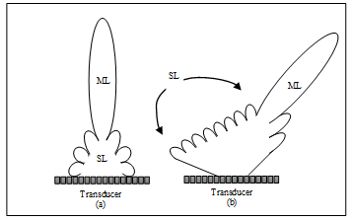Figure 1: (a) Main Lobe (ML) and Side Lobe (SL) of a vertical beam. (b) Main Lobe (ML) and Side Lobe (SL) of a directed beam.

2.2. Dynamic Triangular Apodization (DTA)

The proposed algorithm calculates the apodization values for each channel of every single imaging point, i.e. at each scan angle and each scan depth. In order to combine both windowing and dynamic aperture growth, the algorithm first calculates the required aperture described by three parameters, H, K and a which are derived from the Cartesian coordinates of the adequate point and the width of the transducer. The second part of the algorithm basically fits a Triangular window inside the aperture, while granting the multi-element transducer (0,K) with the maximum weight. zeros are simply assigned to the elements falling outside the aperture. After compressing the apodization values in [0.5, 1] range, all the points that was located at the same direction, will exhibits the same DTA window, hence, the same apodization values. Figure 2 shows the apodization window directivity for two angles, 0° and 5°.

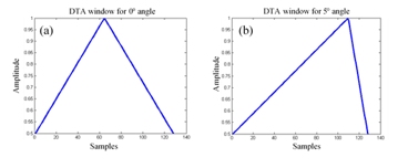Figure 2: (a) Shape of the DTA window for 0° angle (b) Shape of the DTA window for 5° angle

The requested algorithm must find for each multi-element transducer the adequate apodization value. The apodization window is modelled with a triangle.  The point M with coordinates (H, K) of plan P, is the top of this triangle. It is also the targeted point to be scanned. The width of the transducer is the base of the triangle. Therefore, for each point of the plan P, the algorithm provides a new triangular window, and hence new apodization values for every multi-element transducer. The working principle is illustrated in Figure 3.

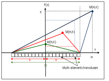Figure 3: Schematic of the dynamic shape of the DTA window

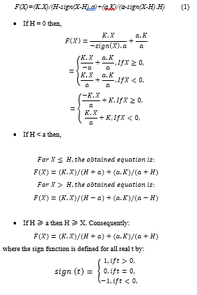
The algorithm solve the problem as follows:

Algorithm 1: DTA algorithm
if  K≥ 0 then        if  H≥ 0 then                if  H = 0 then                      if  X ≥ 0 then                                      F(X) = (-K / a).X+K;                      else if  X < 0 then                                      F(X) = (K / a).X+K;                       end                else if  H < a then                      if  X  H then                                      F(X) = (K/(H+a)).X+(a.K)/(H+a);                      else if  X > H then                                      F(X) = (K/(H-a)).X+(a.K)/(a-H);                                                          end                 else if  H≥ a then                                      F(X) = (K/(H+a)).X+(a.K)/(H+a);                 end        else if  H< 0 then                                      G(X) = – F(X);        end end

where:

• H is the abscissa of the point to be processed
• K is the ordinate of the point to be processed
• X is the abscissa of the transducer elements (referring to their length and position)
• a is the length of half aperture of the transducer

In order to simplify the implementation, the proposed algorithm was alleviated by reducing computational complexity and avoiding potential cumbersome circuits. Therefore, the whole apodization equations mentioned above can be summarized in only one equation described by the following code.

In order to keep the apodization values within the interval [0.5, 1], the final equation Y(X) of the DTA algorithm becomes:

                     

2.3. DTA-Hann approach

To take the advantages of both non-linear and linear apodization techniques, the combination of DTA with the Hanning window was suggested. As a consequence, apodization values for the different multi-element transducers for the same aperture are obtained from DTA and Hanning window, each of them contributing by 50%. The new approach is called DTA-Hann. Figure 4 shows the apodization window directivity obtained with DTA, Hanning and DTA-Hann for 128 multi-element transducers.

The Hanning window is defined by:

Where N is the number of multi-element transducers.

Therefore,  D(X) = (W(X) + Y(X) ) / 2, is the final equation of the DTA-Hann algorithm.

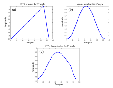Figure 4: (a) Shape of the DTA window for 5° angle (b) Shape of the Hanning window for 5° angle (c) Shape of the DTA-Hann window for 5° angle

2.4. Simulation Setup Configuration

Each of the point spread functions and the cyst phantoms are modelled. All the simulations are implemented in a virtual ultrasound scanning software called Field_II. In the ultrasound software simulator [10], RF (Radio Frequency) echo data are produced using a 1D phased array transducer, which is composed of 128 elements. Each element is characterized by a length of 193 μm, a height of 5 mm, a width of 183 μm and a kerf between adjacent elements of 10 μm. This transducer is able to scan a sector of 60° using a speed of sound of 1540 m/s. Through transmission, the transducer generates a Hanning-windowed 2-cycle sinusoid which bursts at 4 MHz. A relative bandwidth of 60% is used in transmission. The returned signals for each channel are sampled at 100 MHz. The RF data are exported to Matlab for beamforming. Dynamic receive focusing is employed in all algorithms. The Hilbert transformation is applied to the raw received RF data to detect the envelope and the logarithmic compression. To prevent a coarse display due to a large image line spacing, a low-pass interpolation was performed to the raw received RF data laterally by a factor of 5. The scan conversion is the last step to form the image. All images are represented over a 60-dB dynamic range.

• Image Quality Metrics

Good image quality is the main challenge in the reconstruction of an ultrasound system. Therefore, it is assumed that good image quality options are the most important factors in the performance evaluation of an ultrasound imager. A precise diagnosis relies heavily on the obtained image quality, which can be characterized in terms of spatial resolution, contrast resolution, and signal to noise ratio.

• Point Spread Function (PSF)

Metrics used to evaluate the quality of the Point Spread Function (PSF) are adopted from different fields such as radar and communications. The most commonly used metric to measure the resolution is the Full Width at Half Maximum (FWHM), while the side lobe performance is usually measured by the Peak Side lobe Level (PSL). In this evaluation, two new performance evaluation metrics for ultrasound imaging are utilized: Full Width at Half Dynamic Range (FWHDR) and Doubled Main-lobe Level (DML). Choosing a metric based on image dynamic range is well justified. Indeed, when the same image is plotted with a larger dynamic range, the image resolution drops. As a consequence, it becomes harder to distinguish between the closely placed scatterers. Therefore, the FWHDR is effectively the same as the FWHM for log-compressed data. The DML corresponds to the level where the projection of point spread function’s (PSF) area at half dynamic range is doubled, which is equivalent to √2 × FWHDR. The DML is based on a search algorithm that finds the point, in terms of dB, where the width of the main lobe plus side lobes ≥√2 ×FWHDR. The DML search algorithm starts from the tip of the main-lobe and moves vertically down [19] . The PSL does neither quantify the main lobe widening nor estimate the proximity of side lobes. However, the DML reflects the main lobe widening and side lobes behaviour. Nevertheless, it does not pick up the near side lobes, which do not reduce the image quality as much as far side lobes, since they are visualized as a part of the image.

• Cyst Phantom

Ten cysts with radiuses varying from 8.5 mm to 2 mm are located at five penetration depths to evaluate the beamformers under the cyst targets. The cyst phantom consists of a collection of point targets, five cyst regions, and five highly scattering regions. This can be used for characterizing the contrast-lesion detection capabilities of an imaging system. The scatterers in the phantom are generated by finding their random position within a volume of 100 x 100 x 10 mm, and then ascribing a Gaussian distributed amplitude to each scatterer. If the scatterer resides within a cyst region, the amplitude is set to zero. Within the highly scattering region, the amplitude is multiplied by 20. The phantoms typically consist of 50,000 scatterers simulated over 128 scan lines. Figure 5 shows the cyst phantom morphology and the position of each cyst.

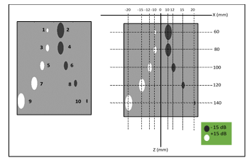Figure 5: Cyst Phantom structures and dimensions

Metrics used to evaluate the quality of the Cyst Phantoms (CP) are:

• Signal to Noise Ratio (SNR)

The system sensitivity and echo detection capability depend on the determination of a system signal-to-noise ratio (SNR). The SNR can be measured using a tissue-mimicking phantom, in which case the SNR as a function of depth, z, can be determined as the ratio of the signal power, S, to the noise power, N [20]:

where E is the expectation operator, and x is the signal RF value.

In this article, the signal power will be estimated from M measurements as:

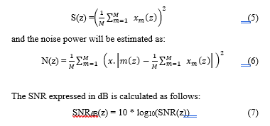penetration depths to evaluate the beamformers under the cyst targets.

• Contrast to Noise Ratio (CNR)

To quantify the contrast in the final image, the Contrast-to-Noise (CNR) values can be used, where the contrast is defined as the logarithmic difference between the mean values of the image kernels fully within and outside the cysts.

The CNR is expressed as [21]:

where μ denotes the mean and σ denotes the standard deviation of the log-compressed B-mode image. The subscripts T and B stand for the target and the background, respectively.

3. Results

3.1. PSF results

Figure 6 shows the Point Spread Function simulation results of DTA, DTA-Hann, Hanning and rectangular apodization algorithms. Results are generated for 6 different steering angles which are 0°, 5°, 10°, 15°, 20° and 25° for points located at the same depth which is 100 mm. Only the right side of the steering is considered, because the results obtained for negative steering angles are symmetric to positive ones.

It can be noticed from the figure that the DTA algorithm and DTA-Hann exhibit better  main lobe characteristics compared to other algorithms. However, the side lobe levels are relatively higher than those obtained with the Hanning window.

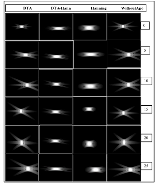Figure 6: Point Spread Function simulation results for 0,5,10,15,20 and 25 steering angles, using three apodization algorithms; DTA, DTA-Hann, Hanning, and without apodization

Table 1 presents the Full Width Half Maximum (FWHM) for axial resolution evaluation of the PSFs. The DTA technique provides excellent results at 0°, 15° and 25° steering angles with 82 μm, 80.4 μm and 82.2 μm respectively. The rectangular apodization also offers some of the best results and shows an optimal main lobe width.

In order to quantify uncertainties between the two most accurate techniques, which are DTA and rectangular window, the Relative Difference (RD) method was calculated in the last column of the table, with the equation:

RD(%)=100×(B- A)/A                                        (9)

 where A and B are two different scenarios. The relative difference shows a very negligible difference between them regarding FWHM for axial resolution. Indeed, the percentage of the difference is within [-3, 3].

Table 1: FWHM Axial Resolution (μm)

Algorithm Angles	A = DTA	DTA-Hann	Hanning	B = Without_apo	RD(%)
0°	82	82	82.9	83.3	1.58
5°	81.6	82.2	82.8	79.7	-2.32
10°	82.4	83.2	81.6	80.5	-2.3
15°	80.4	82.3	83.2	82.7	2.86
20°	81.5	83.8	82.1	80.5	-1.22
25°	82.2	82.5	83.3	81.9	-0.36

Table 2 presents the Peak Side Lobe (PSL) for axial resolution evaluation of the four algorithms. The Hanning window shows the best values for all simulations. It exhibits the smallest levels of PSL. The DTA-Hann window also gives optimal PSL values, a little bit higher than Hanning results. The DTA algorithm offers PSL values very close to those provided by rectangular apodization.

Contrary to the FWHM, the relative difference obtained between the two most accurate techniques, which are DTA-Hann and Hanning window in this case, shows an important difference between them regarding PSL for axial resolution. The difference increases for large opening angle.  Therefore, the Hanning window is more performant in the suppression of side lobe levels.

Table 2: PSL Axial Resolution (dB)

Algorithm Angles	A = DTA	DTA-Hann	Hanning	B = Without_apo	RD(%)
0°	-320.36	-397.62	-436.18	-289.75	9.69
5°	-309.51	-309.12	-383.61	-312.27	24.09
10°	-326.20	-363.04	-678.30	-344.25	86.84
15°	-306.23	-345.35	-675.75	-319.92	95.65
20°	-274.49	-315.76	-672.48	-288.89	113
25°	-217.74	-265.18	-323.27	-229.36	21.62

Table 3 details the PSF performance for axial resolution. It shows the FWHDR image quality option. The best parameters for each apodization algorithm are highlighted in the table below. The best performances are obtained for the DTA and rectangular windows. Obviously, the DTA apodization gives a wider FWHDR than the rectangular window, for 0°, 15° and 25° angles, indicating a better image resolution.

The last column of Table 3 shows the relative difference between DTA and rectangular window. The difference is very negligible regarding FWHDR for axial resolution. In fact, the percentage of the difference is within [-3, 1].

Table 3: FWHDR Axial Resolution (μm)

Algorithm Angles	A = DTA	DTA-Hann	Hanning	B = Without_apo	RD(%)
0°	171.0	171.0	171.5	172.4	0.8
5°	168.2	172.0	171.8	163.1	-2.9
10°	165.1	172.2	170.9	163.4	-1.0
15°	169.6	171.4	172.2	170.9	0.76
20°	171.1	173.0	171.6	168.2	-1.69
25°	166.9	172.4	172.7	168.5	0.95

Table 4 details the PSF performance for axial resolution. It shows the DML image quality option. The best performances are obtained with the DTA-Hann and Hanning windows. Therefore, the DTA-Hann technique provides better main lobe characteristics than the Hanning, for 10° and 20° angles, indicating a better image resolution especially for more deviated directions.

The relative difference obtained between the two most accurate techniques, which are DTA-Hann and Hanning window, shows a little difference between them regarding DML for axial resolution. Therefore, both techniques are suitable in this case.

Table 4: DML Axial Resolution (μm)

Algorithm Angles	A = DTA	DTA-Hann	Hanning	B = Without_apo	RD(%)
0°	-68.6	-68.6	-69.4	-70.3	1.16
5°	-68.1	-68.9	-69.7	-65.9	1.16
10°	-66.7	-69.1	-68.5	-66.1	0.86
15°	-68.1	-68.5	-69.7	-68.9	1.75
20°	-69.1	-69.3	-68.5	-67.5	1.37
25°	-65.5	-68.5	-69.4	-66.9	1.31

Table 5 presents the Full Width Half Maximum (FWHM) for lateral resolution evaluation of the PSFs generated by the four apodization techniques. Obviously, the DTA and DTA-Hann algorithms provide in this case the best values of FWHM. These results are optimal for an ultrasound imaging application. The rectangular apodization shows very close FWHM values. However, the Hanning gives very large FWHM lateral resolution values, especially for a very large opening angle.

Table 5: FWHM Lateral Resolution (μm)

Algorithm Angles	A = DTA	DTA-Hann	Hanning	B = Without_apo	RD(%)
0°	48	44.5	68.2	49.6	3.33
5°	44	52.8	68.8	33.5	-23.86
10°	36.6	53.6	69.3	34.2	-6.55
15°	50.5	47.2	71.2	50.1	-0.79
20°	51	52.1	73.6	43.0	-15.68
25°	43.6	56	76.7	43.3	-0.68

The relative difference between the most accurate techniques, which are DTA and rectangular window, is more or less significant regarding FWHM for lateral resolution. The rectangular window provides better main lobe especially for 5° and 20°.

Table 6 presents the Peak Side Lobe (PSL) for lateral resolution evaluation of the four algorithms. The Hanning and DTA-Hann window show the best values for almost all simulations, with a little difference between them. They exhibit the smallest levels of PSL lateral resolution. The DTA algorithm provides acceptable values for less deviated angles (0°, 5° and 10°), but values at higher steering angles are very similar to those of rectangular apodization.

An important difference appears between the two best techniques regarding PSL for lateral resolution, which are DTA-Hann and Hanning window. The difference increases for large opening angle. Consequently, the Hanning window is more performant in the suppression of side lobe levels. However, only for 10° opening angle, the DTA-Hann gives better results than Hanning.

Table 6: PSL Lateral Resolution (dB)

Algorithm Angles	A = DTA	DTA-Hann	Hanning	B = Without_apo	RD(%)
0°	-381.22	-335.85	-377.52	0	12.40
5°	-137.22	-375.38	-454.77	-142.94	21.14
10°	-145.81	-346.99	-216.21	-149.02	37.68
15°	-121.32	-203.59	-558.17	-124.07	174.16
20°	-120.20	-317.82	-579.26	-124.83	114.07
25°	-121.47	-198.54	-586.63	-125.03	195.47

Table 7 presents the FWHDR performance for lateral resolution of the PSF.  Obviously, the DTA technique exhibits a very similar profile to the rectangular windowing technique. However, the DTA apodization gives a wider FWHDR for 15° angle.

The relative difference between the two best techniques, which are DTA and rectangular window, reveals an important difference between them for less deviated angles. The FWHDR lateral resolution provided by DTA is better for highly deviated angles.

Table 7: FWHDR Lateral Resolution (μm)

Algorithm Angles	A = DTA	DTA-Hann	Hanning	B = Without_apo	RD(%)
0°	102.4	121.1	149.1	93.2	-8.98
5°	96.6	117.0	152.1	81.5	-15.63
10°	86.4	115.3	153.7	82.1	-4.97
15°	95.2	120.6	156.8	95.4	0.21
20°	99.6	123.1	162.2	94.6	-5.02
25°	100.8	125.6	169.1	100.2	-0.59

Table 8: DML Lateral Resolution (μm)

Algorithm Angles	A = DTA	DTA-Hann	Hanning	B = Without_apo	RD(%)
0°	-63.8	-60.9	-55.8	-71.0	11.28
5°	-63.9	-62.4	-58.6	-56.9	-10.95
10°	-57.7	-64.7	-58.8	-56.5	-2.07
15°	-70.3	-61.8	-56.5	-71.0	0.99
20°	-68.2	-61.6	-58.6	-62.8	-7.91
25°	-58.2	-56.2	-58.6	-59.0	1.37

Table 8 describes the DML performance for lateral resolution of the PSF. Also here, the DTA and rectangular windowing techniques provide the best performances. In addition, the DTA apodization shows the best profile for 5° and 20° angles.

A little difference is obtained between the two most accurate techniques regarding DML for lateral resolution, which are DTA and rectangular window. As a consequence, the two techniques are similar in this case.

3.2. Cyst Phantom Results

The reconstructed images are provided in Figure 7. Obviously, the cyst targets are not easily detected in the image generated by rectangular apodization. Moreover, the reconstructed images suffer from the noise. Indeed, the DTA-Hann technique results in a higher quality image and more detectable cyst targets.

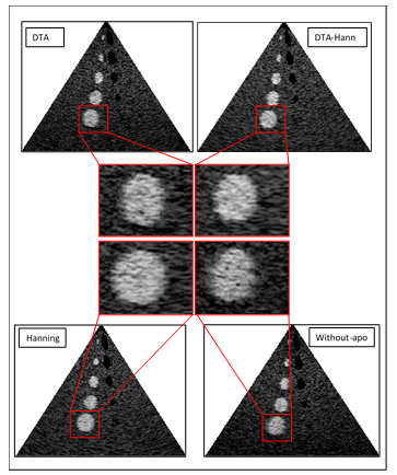Figure 7: Cyst Phantom simulations results for three apodization algorithms; DTA, DTA-Hann, Hanning and without apodization.

Table 9 presents the Signal to Noise Ratio (SNR) and Contrast to Noise Ratio (CNR) evaluation of the cyst phantom technique for three apodization algorithms; DTA, DTA-Hann, and Hanning, as well as the algorithm without apodization. The best SNR is obtained with the DTA method, reaching 14.34 dB. The rectangular apodization also provides acceptable SNR values with 14.32 dB. However, the DTA-Hann and Hanning methods show lower SNR values with 13.98 dB and 13.88 dB, respectively.

The CNR results demonstrate that the DTA and DTA-Hann methods offer the best values, which are 42.42 dB and 42.66 dB, respectively. The Rectangular apodization and Hanning apodization show less accurate CNR results, with 41.35 dB and 42.25 dB, respectively.

A little difference is obtained between the two most accurate techniques regarding CNR and SNR (RD = -056% for CNR and RD = 2.57% for SNR), which are DTA and DTA-Hann. Consequently, the two techniques are similar in this case.

Table 9: Signal to Noise Ratio (SNR) and Contrast to Noise Ratio (CNR) evaluation of the cyst phantom

Apodization Type	SNR (dB)	CNR (dB)
B = DTA	14.34	42.42
A = DTA-Hann	13.98	42.66
Hanning	13.88	42.25
Without	14.32	41.35
R D (%)	2.57%	-0.56%

4. Discussion

The dual apodization technique DTA-Hann offers excellent image quality, which is revealed by PSF and Cyst phantom simulation results. For tissue structures located at less deviated angles, the DTA gives results very close to those obtained with linear windows. For tissue structures located at more deviated angles, the DTA-Hann provides the best image quality in terms of SNR and CNR. This is due to the fact that DTA-Hann eliminates the side lobes produced by the field generated in the same directivity. The DTA-Hann algorithm gives an optimal FWHM compared to Hanning and rectangular windows. Indeed, this is justified by the high selectivity of the undamaged transmitted and received echoes. However, the PSL levels are relatively high especially for very deviated angles, and this is generated because of the non-linearity of the dynamic algorithm.

When DTA-Hann and Hanning algorithms are compared qualitatively and quantitatively as shown in Figure 7 and Table 10, the FWHM shows a relative difference of 29.29% between them  (DTA-Hann: scenario A with 53.6 µm, Hanning: scenario B with 69.3 µm). In fact, the scenario A is much better than the scenario B.  The scenario A provides 130 dB and 5.9 dB more than the scenario B in terms of PSL and DML, respectively. When the FWHDR is used to measure the lateral width, there is a difference of 33.3% between these two cases (A = 115.3 µm, B = 153.7 µm). Here also, the scenario A is much better than the scenario B.

Table 10: Performance metrics comparison for lateral resolution at 10° angle between DTA-Hann and Hanning windows

	FWHM	FWHDR	DML	PSL
A = DTA-Hann	53.6	115.3	-64.7	-346.99
B = Hanning	69.3	153.7	-58.8	-216.21
RD(%)	29.29 %	33.30%	-9.11%	37.68%

The DTA-Hann technique is more selective than linear functions, providing the best main lobe characterization. Side lobes reductions are more or less significant using DTA-Hann since they depend on the deviation angle. Linear methods are more efficient for side lobes elimination, but at the cost of less characterization of the main lobe.

Finally, the DTA-Hann algorithm is more suitable to ultrasound imaging than linear apodization windows.  It is the most performant and selective. It also offers the most accurate image options for cyst phantom simulation.

The DTA is used in transmit and receive apodization. Dynamic receive apodization methods are possible and can be implemented easily in the digital beamforming ultrasound software. However, dynamic transmit apodization methods are not very known for the time being, and the exploration of the DTA-Hann in transmission is among prospects of future work for more evaluation and study.

5. Conclusion

In this paper, a new dynamic apodization technique (DTA) that enables windowing for each imaging direction was proposed. Then, the efficiency of a non-linear windowing technique that combines the Hanning window with the DTA algorithm was evaluated.

In the point target simulation, the main lobe widths of the dual-apodization algorithm were very similar to those of the rectangular window without removing side lobes. In the cyst target simulation, CNR values of the dual apodization were significantly improved. The Dynamic Triangular Apodization is our new suggested method. It is based on following the shape of the transmitted and received ultrasound field from a focal point. Thanks to this method, the apodization weight becomes more sensitive to the undamaged transmitted and received echoes. This apodization method can be used in transmission and reception. Actually, the implementation of the DTA-Hann algorithm in digital beamforming ultrasound software is among prospects of future work.

Conflict of Interest

The authors declare no conflict of interest.

1. K. Sumaiya, S.S. Kawathekar, “Drawbacks of Poor-Quality Ultrasound Images and its Enhancement,” International Journal of Computer Applications, 175, 47–55, 2020, doi:10.5120/ijca2020920880.
2. A. Ilovitsh, T. Ilovitsh, K.W. Ferrara, “Multiplexed ultrasound beam summation for side lobe reduction,” Scientific Reports, 9(1), 13961, 2019, doi:10.1038/s41598-019-50317-7.
3. A. Agarwal, J. Reeg, A.S. Podkowa, M.L. Oelze, “Improving Spatial Resolution Using Incoherent Subtraction of Receive Beams Having Different Apodizations,” IEEE Transactions on Ultrasonics, Ferroelectrics, and Frequency Control, 66(1), 5–17, 2019, doi:10.1109/TUFFC.2018.2876285.
4. A.N. Madhavanunni, M.R. Panicker, “Directional Beam Focusing Based Dual Apodization Approach for Improved Vector Flow Imaging,” in 2020 IEEE 17th International Symposium on Biomedical Imaging (ISBI), 300–303, 2020, doi:10.1109/ISBI45749.2020.9098494.
5. A. Vayyeti, A.K. Thittai, “A Weighted Non-Linear Beamformer for Synthetic Aperture Ultrasound Imaging,” in 2020 IEEE International Ultrasonics Symposium (IUS), 1–3, 2020, doi:10.1109/IUS46767.2020.9251413.
6. J.T. Yen, E. Powis, “Boundary Array Transducer and Beamforming for Low-Cost Real-time 3D Imaging,” in 2020 IEEE International Ultrasonics Symposium (IUS), 1–4, 2020, doi:10.1109/IUS46767.2020.9251670.
7. Side lobe free medical ultrasonic imaging with application to assessing side lobe suppression filter | SpringerLink, Sep. 2021.
8. W. Guo, Y. Wang, J. Yu, “A Sibelobe Suppressing Beamformer for Coherent Plane Wave Compounding,” Applied Sciences, 6(11), 359, 2016, doi:10.3390/app6110359.
9. S. Lu, R. Li, Y. Zhao, X. Yu, D. Wang, M. Wan, “Dual apodization with cross-correlation combined with robust Capon beamformer applied to ultrasound passive cavitation mapping,” Medical Physics, 47(5), 2182–2196, 2020, doi:10.1002/mp.14093.
10. Sidelobe reduction for plane wave compounding with a limited frame number | BioMedical Engineering OnLine | Full Text, Sep. 2021.
11. A. Ibrahim, P.A. Hager, A. Bartolini, F. Angiolini, M. Arditi, J.-P. Thiran, L. Benini, G. De Micheli, “Efficient Sample Delay Calculation for 2-D and 3-D Ultrasound Imaging,” IEEE Transactions on Biomedical Circuits and Systems, 11(4), 815–831, 2017, doi:10.1109/TBCAS.2017.2673547.
12. W. Hechkel, B. Maaref, N. Hassen, “Evaluation of transmit/receive apodization scheme for hardware implementation used in B-mode ultrasound imaging,” in 2020 17th International Multi-Conference on Systems, Signals Devices (SSD), 808–813, 2020, doi:10.1109/SSD49366.2020.9364236.
13. W. Hechkel, B. Maaref, N. Hassen, “Evaluation of a novel ultrasound imaging methods for high frame rate echocardiography,” in 2020 17th International Multi-Conference on Systems, Signals Devices (SSD), 185–190, 2020, doi:10.1109/SSD49366.2020.9364257.
14. W. Hechkel, B. Maaref, N. Hassen, “New Sector Scan Geometry for High Frame Rate 2D-Echocardiography using Phased Arrays,” International Journal of Advanced Computer Science and Applications (IJACSA), 11(12), 2020, doi:10.14569/IJACSA.2020.0111266.
15. G. Malamal, M.R. Panicker, “Towards A Pixel-Level Reconfigurable Digital Beamforming Core for Ultrasound Imaging,” IEEE Transactions on Biomedical Circuits and Systems, 14(3), 570–582, 2020, doi:10.1109/TBCAS.2020.2983759.
16. M. Agarwal, A. Tomar, N. Kumar, “An IEEE single-precision arithmetic based beamformer architecture for phased array ultrasound imaging system,” Engineering Science and Technology, an International Journal, 24(5), 1080–1089, 2021, doi:10.1016/j.jestch.2021.03.005.
17. J.T. Yen, M.M. Nguyen, Y. Lou, J.S. Shin, Y. Chen, H.L. Tarnoff, “Gated Transmit and Fresnel-Based Receive Beamforming With a Phased Array for Low-Cost Ultrasound Imaging,” IEEE Transactions on Ultrasonics, Ferroelectrics, and Frequency Control, 68(6), 2183–2192, 2021, doi:10.1109/TUFFC.2021.3062850.
18. R.J.G. van Sloun, R. Cohen, Y.C. Eldar, “Deep Learning in Ultrasound Imaging,” Proceedings of the IEEE, 108(1), 11–29, 2020, doi:10.1109/JPROC.2019.2932116.
19. S. Harput, J. McLaughlan, D.M.J. Cowell, S. Freear, “New performance metrics for ultrasound pulse compression systems,” in 2014 IEEE International Ultrasonics Symposium, 440–443, 2014, doi:10.1109/ULTSYM.2014.0109.
20. V. Papic, Z. Djurovic, G. Kvascev, P. Tadic, “On signal-to-noise ratio estimation,” in Melecon 2010 – 2010 15th IEEE Mediterranean Electrotechnical Conference, 160–165, 2010, doi:10.1109/MELCON.2010.5476314.
21. M. Welvaert, Y. Rosseel, “On the Definition of Signal-To-Noise Ratio and Contrast-To-Noise Ratio for fMRI Data,” PLOS ONE, 8(11), e77089, 2013, doi:10.1371/journal.pone.0077089.

(Click Here)