1. Introduction

This research is an extended version of the work presented at the 2020 IEEE 2nd International Conference on System Analysis_Intelligent Computing (SAIC) held in Kyiv, Ukraine, in October 2020 [1] as well as the consequently published paper [2] from the Advances in Science, Technology and Engineering Systems Journal in May 2021. These papers reported that a rotating object would produce anti-gravity, if it held a heavy mass that would distort time and space. The last paper [2] informed of the waves emitted from the rotating object; however, the report of the analysis was forwarded to this new paper because the numeric simulation required a separate research.

An explicit image of the anti-gravity of the rotating object is a flying craft having a disc-shaped body for interstellar travel. Such an object should hold a compact nuclear fusion reactor inside, because the fusion reaction forms the heavier nuclei by fusing the lighter ones such as hydrogen, deuterium and tritium, and this process should distort time and space. However, this is the theory of a black hole [3], and the simulation of the time-space distortion in the nuclear fusion reactor is still the topic of the next research after this paper.
The waves emitted from the source of the anti-gravity are byproducts, but they can indicate the presence of the source if they have any physical properties such as the energy intensity and the spin angular momentum. The goal of this research is to calculate the energy intensity and the angular momentum of the waves.
In order to describe this phenomenon, the 4-dimensional curvilinear coordinates of the curved space are selected because the heavy object should warp the rectilinear coordinates of the flat space. To start the simulation, the curvature tensor, Rμν, is given to describe time and space where the object with a heavy mass is placed [3].

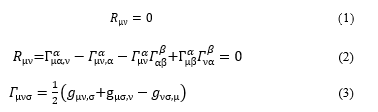
This curvature tensor includes the first-order differentials of a fundamental tensor (gμν), gμν,σ = ∂gμν/∂xσ, where xσ is the σ-th vector (variable) in the given coordinates. Before describing the phenomenon in the curvilinear coordinates, the flat space provides a significant introduction to the theory of the waves. Therefore, at first a series of the notations derives the tensor of the waves in an approximate flat space in this introductory section, and then the tensor of the waves is derived in the curved space later in the next section 2.1.
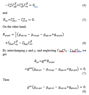
If the gravitational field is weak, the curvature is also weak and gμν is approximately constant; therefore,

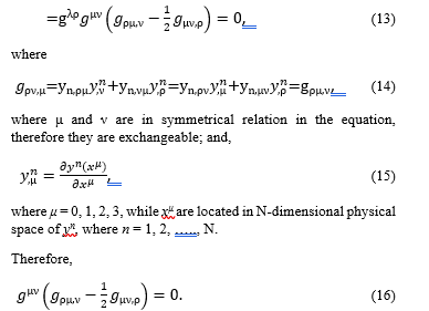
In order to describe a particle moving in the 4-dimensional time and space, V is replaced by vectors xλ of the 4-dimensional coordinates in which xλ,α = gλα,, then d’Alembert equation becomes

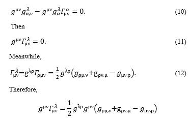
Therefore,

Then, in order to describe the waves moving in the gravitational field, it is differentiated by xσ.

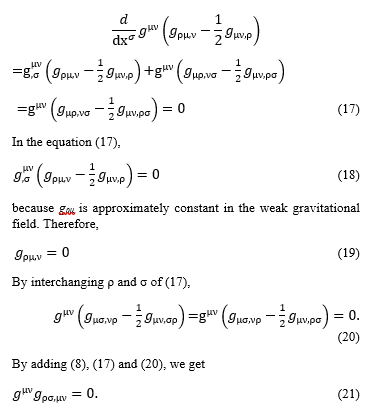
It satisfies d’Alembert equation, therefore it describes the waves that move in an empty space where there is only the weak gravitational field. (Note: This equation includes the second-order differentials, gμν,ρσ = ∂2gμν /∂xρ∂xσ.)
The equation (21) describes the waves moving in the weak gravitational field that is approximately a flat 4-dimensional time and space; however, the general theory of relativity predicts the flow of the waves in curvilinear coordinates of the stronger gravitational field. In order to simulate the flow of the waves in the stronger gravitational field, this research includes the following terms that have been neglected in the classic reference [3]:

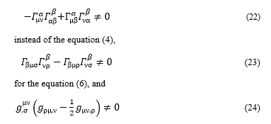
instead of the equation (18).
In this research, the energy intensity and the spin angular momentum of the flow of the waves are simulated as the calculated coefficients of the tensor equation in the spherical polar coordinate system, which is one of the curvilinear coordinate systems. The methodology and the result of the simulation are reported in the following sections.

Methodology

Algorithm

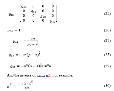For the research of the strong gravitational field, gμν, is not constant, but given by the following matrix, [3]:
Then t is time, m is the mass of the object, r is the distance from the center of the object, θ is the angle between r and the rotation axis, z, and ϕ is the angle of the rotation around the rotation axis in the spherical polar coordinates shown in Figure 1.
τ is the distorted time and ρ is the distorted distance as defined by the following equations [3].
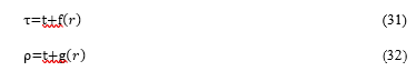
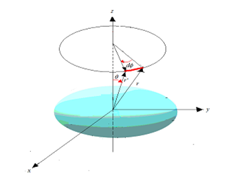Figure 1: Spherical polar coordinates for the simulation

 

f(r) and g(r) are the functions later defined in the section 2.2. μ is given by the following equation with the mass, m, of the object ([3] p. 35):

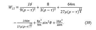
The equations below from (34) to (38) show how to derive the equation of the waves in the curved space. It follows the same logic from (7) to (21) in the introductory section above, which derives the equation of the waves in the approximate flat space. But, the equations below include the neglected terms in order to derive the equation in the curved space.
By adding the neglected terms of the equation (23) to the equation (7), we get:

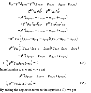
By adding the neglected terms to the equation (17), we get

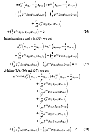
The equation (38) describes the waves that move in the strong gravitational field. The numbers, 0, 1, 2, and 3, are assigned to each of μ, ν, ρ, σ and β of the equation (38); then by the rule of tensor, all terms are summed up. Then the mathematical forms of the equation (38) are derived by the functions shown in the equations from (26) to (29). Then according to the equation (25), non-diagonal components such as g12 and g23 vanish; then only diagonal components remain as shown in the equations from (39) to (41). Hereinafter this research focuses on the spatial distribution of the waves but doesn’t consider the time. Time is taken into account only by the distorted distance, ρ, of the equation (32). Therefore, only three diagonal components of a 3×3 matrix that represent the spatial distribution of the waves are considered.

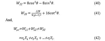
16μ3/18m of the equation (39) is a constant term, and it is not included in the equation (42) for the simulation.
The algorithm to simulate the relative energy intensity of the waves is as follows:
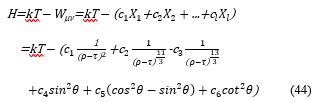
It is assumed that the stress energy tensor, T, reflects the energy intensities of the waves as shown in the equation (43), where k is a constant.

The idea of the stress energy tensor is taken from the classical mechanics [4] (p. 327).
Each of the coefficients, c1, c2 ··· cl, relates to a component of the waves such as 1/(ρ-τ)2, 1/(ρ-τ)3/11, and so on. With the equation (44) we calculate the coefficients, c1, c2 ··· cl.

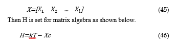
These coefficients make a column vector, c, which holds l rows. For calculating c, X (a n×l matrix) is set as shown in (45), where each of X1, X2, ··· Xl is a vector that holds n rows, and n is also the number of rows of each column of X. In this simulation the value of n is 23 as later explained in the section of the input data, and l is 6 for the equation (44).
The vectors of the matrix X should hold the projected image of the energy intensity on the surface of the sphere in the spherical polar coordinates. (Note: The surface of the sphere refers to Figure 14 of [2].

To solve this equation, a constraint is given as shown below, where X’ is the transposed matrix of X.

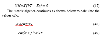
here (X’X)-1 is an inverse matrix of X’X.
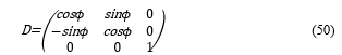
If the object rotates as shown in Figure 1, its coordinate system is transformed by the transformation matrix D of the Euler’s angles [4] as shown below.

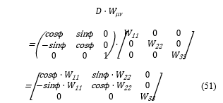
To simulate the rotation of the object around the axis of z, the matrix, Wμν, is multiplied by D; then it is transformed as shown below.

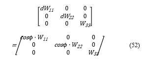
To calculate the energy intensity of the waves, the diagonal components are taken from the above transformed matrix, D·Wμν, then a matrix (52) is set.

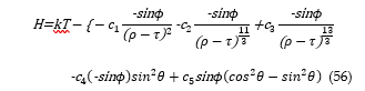
Then an equation of H is set as shown below to calculate the coefficients of the diagonal components.

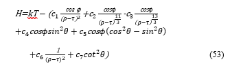
Hereinafter the same procedure follows as explained from the equation (44) to (49) to calculate the coefficients.
To calculate the spin angular momentum, a matrix is set as shown in (54), by taking out the anti-symmetrical components of D·Wμν from (51).

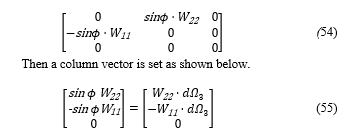
With the above column vector, an equation of H is set as shown below for the calculation of the coefficients.

The spin angular momentum is to be projected on the flat surface, which is perpendicular to the curved spherical surface in the spherical polar coordinate system. (Note: The flat surface refers to Figure 15 of [2].
Input data
Figure 2 and Figure 3 show the input data that simulate the distortion of time and space, which we used also for the previous research [1, 2]. In these figures, r is the distance from the center of the strong gravity; t is the time to travel for the distance; τ is the distorted time by the equation (31), which expands and shrinks depending on r and t; and, ρ is the distorted distance by the equation (32), which expands and shrinks depending on t and r.

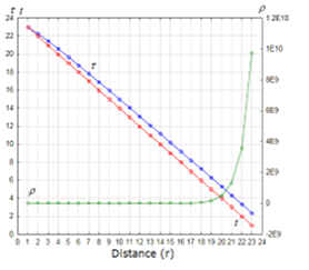Figure 2: Time and distance from the center of the gravity, Case-1 (non-linear model): f(r)=log r and g(r)= er

 

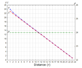Figure 3: Time and distance from the center of the gravity, Case-2 (linear model): f(r) = 1/r and g(r) = r

For the distorted time and space, two models are set: Case-1 (non-linear model) and Case-2 (linear model) as shown in Table 1, which assign the functions of f(r) of the equation (31) and g(r) of the equation (32).
Table 1: Two models for simulating the distorted time-space

	Case-1 (Non-linear model)	Case-2 (Linear model)
f(r)	log·r	1/r
g(r)	er	r

Then the distributions of r and t are set to simulate the description of the reference [3], “Any signal, even a light signal, would take an infinite time to cross the boundary of a black hole”. In our research the term, a black hole, is replaced by the strong gravity that distorts time and space. However it is not possible to set the infinite value for the numeric simulation of this research that uses a personal computer. Therefore we used 24 discrete finite values as the surrogate that simulates “It takes more time to travel closer to the center of the strong gravity”.
The time, t, and the distance, r, are set as shown in Figure 2 for Case-1 and Figure 3 for Case-2. For simulating the waves, we assumed that θ would become smaller in far distance from the object as shown in Figure 4, because the spin of the waves should stabilize the flow as the waves move forward from the center of the gravity; then the angle θ should be focused and smaller in the far distance.
For simulating the rotation of the object, two modes of the frequencies are set: ϕ1 (rotation 1) and ϕ2 (rotation 2) also as shown in Figure 4. The frequency ϕ2 is higher than ϕ1; therefore, rotation 2 represents the faster rotation of the object than rotation 1. With these settings, sin θ, cos θ, cot θ, sin ϕ1,, sin ϕ2, cos ϕ1 and cos ϕ2 change their values as shown in Figure 5.
The value of the stress energy tensor is set as 1; therefore, this simulation doesn’t calculate absolute values of the intensities, but relative intensities. The calculated coefficients have dimensions. For example, the coefficient of the first term of the equation (39), 16/{9(ρ – τ)2}, has the dimension of the inverse of (ρ – τ)2 that is the squared dimension of the difference between the distorted distance, ρ, and the distorted time, τ.

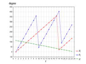Figure 4: Angles, θ, ϕ1 and ϕ2 for the simulation

 

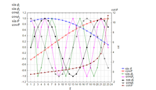Figure 5: Trigonometric functions, sin θ, cos θ, cot θ, sin ϕ1,, sin ϕ2, cos ϕ1 and cos ϕ2 for the simulation

Result

Energy intensity of the waves
The calculated energy intensities of the waves are shown in Table 2 for Case-1 (non-linear model) and Table 3 for Case-2 (linear model). The first and the third columns of these tables are the mathematical forms of the components of the waves, which are taken from the equations from (39) to (41), but each of the constant factors is simplified to unity. For example, 16/{9(ρ–τ)2} is simplified to 1/(ρ–τ)2 because the factor, 16/9, is not necessary as it is to be included in the coefficient when it is calculated by the equation (49).
The calculated coefficients have either positive or negative values. For example, in Case-1 (non-linear model) the calculated coefficient of 1/(ρ–τ)2 is 4.081·10–6 with no rotation; and, it changes to –1.465·104 with rotation 1, and then 4.178·103 with rotation 2. It suggests that the energy intensity of this component of the waves changes its sign from negative to positive when the object rotates faster from rotation 1 to rotation 2.
In order to interpret the calculated results, hereinafter we define that the positive flow holds positive (+) coefficient, and the negative flow holds negative (‒) coefficient. For example in the above case of 1/(ρ–τ)2, the wave is a negative flow with rotation 1; but, it changes to a positive flow with rotation 2.
Table 2: Results of the simulation of energy intensity of the waves, Case-1

Components of Waves (No rotation)	Coefficients (No rotation)	Components of Waves with the rotation	Coefficients (Rotation 1)	Coefficients (Rotation 2)
1/(ρ–τ)2  *	4.081·10–6	cosϕ/(ρ–τ)2	–1.465·104	4.178·103
1/(ρ–τ)11/3	–1.892·10–4	cosϕ/(ρ–τ)11/3	1.682·105	–2.311·105
–1/(ρ–τ)13/3	–3.270·10–4	–cosϕ/(ρ–τ)13/3	2.836·105	–4.028·105
sin2θ	2.000	cosϕsin2θ	8.397·10–2	3.875·10–2
cos2θ–sin2θ	1.000	cosϕ(cos2θ–sin2θ)	1.436	–6.610·10–2
–	–	1/(ρ-τ)2  ⁑	1.041·104	3.825·102
cot2θ	-4.358·10–10	cot2θ ⁑	7.534·10–2	8.819·10–2

Notes for Table 2 and 3.
*: This component belongs to both W11, (16/9(ρ–τ)2 + 8/3(ρ–τ)2, of the equation (39) and W33, (128/9(ρ–τ)2, of the equation (41).
⁑: These components are on the axis of the rotation and belong to W33; therefore, cosϕ is not multiplied.
Table 3: Results of the simulation of energy intensity of the waves, Case-2

Components of Waves (No rotation)	Coefficients (No rotation)	Components of Waves with the rotation	Coefficients (Rotation 1)	Coefficients (Rotation 2)
1/(ρ-τ)2  *	–1.563·10–7	cosϕ/(ρ-τ)2	–17.34	–63.97
1/(ρ–τ)11/3	2.206·10–6	cosϕ/(ρ-τ)11/3	–1.313·102	1.156·103
–1/(ρ–τ)13/3	2.493·10–6	–cosϕ/(ρ–τ)13/3	–1.460·102	1.390·103
sin2θ	2.000	cosϕsin2θ	0.1066	6.768·10–2
cos2θ–sin2θ	1.000	cosϕ(cos2θ–sin2θ)	0.4353	–0.5905
–	–	1/(ρ-τ)2  ⁑	28.03	12.58
cot2θ	–4.306·10–10	cot2θ ⁑	8.474·10–2	8.236·10–3

The summations of the values of each of the positive coefficients and the negative coefficients are shown in Table 4 for both Case-1 and Case-2, and Figure 6 for Case-1 and Figure 7 for Case-2. In both cases, positive and negative flows of the waves are not visible in the figures when the object doesn’t rotate; but, they become visible when the object rotates.
Table 4: Energy intensities of positive and negative flows

	Positive flow	Negative flow
No rotation (Case-1)	3.000	–4.358· 10-10
Rotation 1  (Case-1)	4.622· 105	–1.465· 104
Rotation 2  (Case-1)	4.560· 103	–6.339 · 105
No rotation (Case-2)	3.000	–1.567 · 10-7
Rotation 1  (Case-2)	2.865· 101	–2.947· 102
Rotation 2  (Case-2)	2.558· 103	–6.456· 101

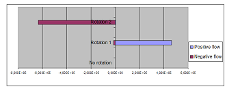Figure 6: Energy intensity of positive and negative flows: (Case-1)

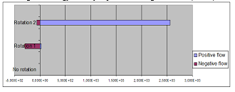Figure 7: Energy intensity of positive and negative flows: (Case-2)

 

Spin angular momentum
Table 5 and Table 6 show the calculated relative intensity of the spin angular momentum of the waves, which are projected in the directions of sinϕ·W22 and -sinϕ·W11. (Note: sinϕ·W22 and -sinϕ·W11 are perpendicular to the rotation axis.)
The calculated coefficients of the spin angular momentum hold either positive or negative signs. For example, in Case-1 (non-linear model) the coefficient of –sinϕ/(ρ–τ)2 is –6.003·103 with the rotation 1, but it changes to 7.215·103 with the rotation 2. –sinϕ/(ρ–τ)2 is one of the projected momenta of 1/(ρ–τ)2 in the direction of -sinϕ·W11, where 1/(ρ–τ)2 represents the first and the second terms of the equation (39), 16/{9(ρ–τ)2 }and 8/{3(ρ–τ)2}.
Then we compare the changes of the spin angular momentum with the changes of the energy intensity. The energy intensity of 1/(ρ–τ)2 in Table 2 for Case-1 (non-linear model) changes its sign from negative to positive when the rotation of the object becomes faster from rotation 1 to rotation 2. It suggests that this component is a negative flow of the waves when the object rotates with the frequency of ϕ1, but when the object rotates faster with the frequency of ϕ2, the waves become a positive flow; and, the spin angular momentum also changes its spinning direction from negative to positive as shown in Table 5.
Table 5: Relative intensity of spin angular momentum, Case-1

Components of the waves	Rotation 1	Rotation 2
–sinϕ/(ρ-τ)2	–6.003·103	7.215·103
–sinϕ/(ρ-τ)11/3	1.400·106	–1.734·106
–sinϕ/(ρ-τ)13/3	4.592·106	–5.688·106
–sinϕsin2θ	–1.163·10–2	–1.234·10–2
sinϕ(cos2θ–sin2θ)	0.2898	–0.5123

Table 6: Relative intensity of spin angular momentum, Case-2

Components of the waves	Rotation 1	Rotation 2
–sinϕ/(ρ-τ)2	–71.08	7.644
–sinϕ/(ρ-τ)11/3	5.946·102	1.031·102
–sinϕ/(ρ-τ)13/3	6.159·102	1.605·102
–sinϕsin2θ	–2.250·10–4	–1.270·10–2
sinϕ(cos2θ–sin2θ)	1.129	–0.5360

The summations of the values for positive and negative coefficients of the spin angular momenta are shown in Table 7 for Case-1 and Case-2, and Figure 8 for Case-1 and Figure 9 for Case-2. In both cases, the values change upon the selection of the rotation-mode of the object, rotation 1 or rotation 2. As shown in the figures, the spin angular momentum changes its sign between rotation 1 and rotation 2 in Case-1 (non-linear model), while such a rule of changing sign is not so clear in Case-2 (linear model).

Table 7: Relative intensity of spin angular momentum

	Positive flow	Negative flow
Case-1 Rotation 1	5.992·106	–6.003·103
Case-1 Rotation 2	7.215·103	–7.421·106
Case-2 Rotation 1	1.212·103	–7.108·101
Case-2 Rotation 2	2.713·102	–5.486·102

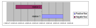Figure 8: Relative intensity of spin angular momentum Case-1

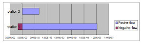Figure 9: Relative intensity of spin angular momentum Case-2

Discussion

The results show that positive and negative flows of the waves appear if the object rotates, and some of the components that indicate positive and negative flows have opposite spinning directions. The results also show that the rotation-mode (rotation 1 or rotation 2) of the object relates to the energy intensity of the emitted waves, as well as their spinning directions.
Table 8 and Table 9 for Case-1 (non-linear model) and Table 10 and Table 11 for Case-2 (linear model) summarize the changes of the signs of the energy intensity and the spin angular momentum.
In Case-1 (non-linear model), except sin2θ, these components change their energy intensities either from positive to negative or from negative to positive, and simultaneously change their signs of the spin angular momenta either from positive to negative or from negative to positive. For example, the component of 1/(ρ–τ)2 is a negative flow with rotation 1, but it is a positive flow with rotation 2; while its spinning direction changes from negative to positive when the rotation-mode changes from rotation 1 to rotation 2.
The coefficients of 1/(ρ–τ)11/3, –1/(ρ–τ)13/3 and cos2θ–sin2θ show the same rule of changing sign, but in the opposite directions of the flow and the spin of 1/(ρ–τ)2 .
This finding in Case-1 (non-linear model) is consistent with Figure 10 of our previous research [5] upon the analysis in rectilinear coordinates, in which the negative flow has the clockwise spin, while the positive flow has the anti-clockwise spin.
The exception, sin2θ, relates to cosϕsin2θ of Table 2 for the energy intensity and to sinϕsin2θ of Table 5 for the spin angular momentum. The absolute values of these calculated coefficients are smaller than those of the other components; and, the flow and the spin don’t change their signs. Therefore this component is not considered significant.
In Case-2 (linear model) shown in Table 10 and Table 11, the rule of changing sign as observed in Case-1 applies only to cos2θ–sin2θ.
Table 8: The sign of the coefficient, energy intensity, Case-1

	No rotation	Rotation 1	Rotation 2
1/(ρ-τ)2	+	–	+
1/(ρ–τ)11/3	–	+	–
–1/(ρ–τ)13/3	–	+	–
sin2θ	+	+	+
cos2θ–sin2θ	+	+	–

Note for Tables 8, 9, 10 and 11: The component of cot2θ doesn’t appear in these tables because it is on the rotation axis, and not considered. 1/(ρ–τ)2 is a simplified form of 16/9(ρ–τ)2 and 8/3(ρ–τ)2; –1/(ρ–τ)11/3 is a simplified form of –64m/27μ(ρ–τ)11/3; sin2θ is a simplified form of 8μ3sin2θ/18m of the equation (39); and cos2θ–sin2θ is a simplified form of 8cos2θ–8sin2θ of the equation (40). All these components are multiplied by cosϕ for calculating the energy intensity and by –sinϕ and sinϕ for calculating the spin angular momentum.
Table 9: The sign of the coefficient, Spin angular momentum, Case-1

	Rotation 1	Rotation 2
–sinϕ/(ρ-τ)2	–	+
–sinϕ/(ρ-τ)11/3	+	–
–sinϕ/(ρ-τ)13/3	+	–
–sinϕsin2θ	–	–
sinϕ(cos2θ–sin2θ)	+	–

Table 10: The sign of the coefficient, energy intensity, Case-2

	No rotation	Rotation 1	Rotation 2
1/(ρ–τ)2	–	–	–
1/(ρ–τ)11/3	+	–	+
–1/(ρ–τ)13/3	+	–	+
sin2θ	+	+	+
cos2θ–sin2θ	+	+	–

Table 11: The sign of the coefficient, Spin angular momentum, Case-2

	Rotation 1	Rotation 2
–sinϕ/(ρ-τ)2	–	+
–sinϕ/(ρ-τ)11/3	+	+
–sinϕ/(ρ-τ)13/3	+	+
–sinϕsin2θ	–	–
sinϕ(cos2θ–sin2θ)	+	–

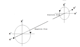Figure 10: Geometrical relation between positive and negative flows in flat space (from [5])

Conclusion and recommendation

The result indicates that the rotation of the object can produce both positive and negative energy intensities of the waves, and they are interpreted as positive and negative flows. Both positive and negative flows appear when the object rotates, although the selection of the input data, the non-linear model or the linear model, leads to differences of the energy intensities.
With the non-linear model, the calculated spin angular momentum of the waves changes its sign, + or ‒, when most of the components change the signs of their energy intensities either from positive to negative or from negative to positive, depending on the speed of the object’s rotation. This finding means that most of the components of the waves change their spinning directions when the energy intensity of the flow of the waves changes its sign + or ‒, also depending on the speed of the object’s rotation. This particular finding on the spin angular momentum is consistent with the previous research [5]. However, with the linear model, most of the components of the waves don’t follow the same rule of changing sign.
A parallel image of the source of the anti-gravity is a rotating black hole, and the same rule may apply. Then the positive flow of the waves may be gravitational waves and the negative flow may be the gravitational waves that flow in opposite directions. If those gravitational waves are observed from a rotating black hole and if they indicate the same rule of the energy intensity and the angular momentum as shown in this paper, it will certify the theory.
On the other hand, the theory of the time-space distortion should be verified with a compact nuclear fusion reactor for developing the flying craft. At the next step of the research, it is necessary to calculate the probability of proton-capture or proton-charge-exchange with the time-space distortion model that is used for the simulation reported in this paper.

1. Y. Matsuki, P.I. Bidyuk, “Theory and Simulation of Artificial Antigravity,” 2020 IEEE 2nd International Conference on System Analysis Intelligent Computing, 2020, doi: 10.1109/SAIC51296.2020.9239195.
2. Y. Matsuki, P.I. Bidyuk, “Numeric Simulation of Artificial Antigravity upon General Theory of Relativity,” Advances in Science, Technology and Engineering Systems Journal, 6(3), 45-53, 2021, doi: 10.25046/aj060307.
3. P.A.M. Dirac, General Theory of Relativity, New York: Florida University, A Wiley Inter-science Publication, John Wiley & Sons, 1975.
4. H. Goldstein, C.P. Poole, J.L. Safko, Classical Mechanics, 3rd Edition published by Pearson Education. Inc., 2002.
5. Y. Matsuki, P.I. Bidyuk, “Analysis of Negative Flow of Gravitational Waves,” System Research & Information Technology, N4, 7-18, 2019, doi: 10.20535/SRIT.2308.8893.2019.4.01.

(Click Here)