1. Motivation

According to the Occupational Safety and Health Administration (OSHA), industry related injuries indicate that from 2015 to 2019, 76% of injuries (4 injuries total) were severe and 3 fatalities occurred throughout the USA [1]. These injuries are attributed to autonomous cars, mobile cars, and AGVs. OSHA states that there were 30 casualties in human-robot workspaces from 1987 to 2019. Due to a significant increase in robot installation worldwide, and the increasing amount of interaction, it has become important to investigate the robot(s) locomotion within workspace, examine the probability of accidents, and determine a solution to minimize unsafe interaction. Automated Guided Vehicle systems (AGVs) provide manufacturing and logistic facilities with added flexibility thereby increasing the overall rate of production. These AGVs are outfitted with appropriate safety equipment and sensors to make them safe while in operation [2]. The main advantage of AGVs are that “if properly guided”, they do not injure people and/or damage infrastructures. It is generally accepted that AGVs are safer than manual equipment such as conventional forklifts. The introduction of collaborative AGVs or robots has initiated the concept of fencing, and currently, in this advanced technology era, the combined work effort between humans and robots has become efficient and productive. However, the coexistence of autonomous mobile robots within themselves and most often in the presence of humans have made safety a priority in a shared workspace. This study is concerned with a worst-case scenario when a robot loses its path planning capability due to a communication or processing malfunction.  The locomotion type discussed in this research assumes random walk for both robot-robot and human-robot interaction. This paper provides literature review on automatic guidance and safety method. The concept of Random Walk is then presented to application of robot locomotion, with a goal to understand efficiency to navigate in absence of a real-time localization system. Extensive computational simulations are performed for several robot interaction with structured and random obstacle in confined area, and with objective to study navigation tradeoff under random walk.

2. Automatic Guidance

AGVs can be used in external and internal environments such as manufacturing, distribution, transhipment and (external) transportation areas [3]. AGVs also play an important role in the transportation of materials that are associated with manufacturing processes. About 20,000 AGVs are utilized for industrial applications [4]. The use of the automated guided vehicle has increased significantly since their introduction. According to [5], the human-machine interfaces facilitate the users to perform coordinated logistical activities within industrial environments. For example, PMD-cameras (Photonic Mixer Device camera) are typically used in sensing the obstacles within the path of an AGV. The PMD-camera acts as an interactive technique that records the video images of various objects and scenes in both 2-D and 3-D greyscales and deep-data images, respectively. In addition, the same technique is used when there is a need to monitor the area where an industry robot is working [6].  According to [7] , human-robot interface systems design considers the formation of a multi-agent framework, thus taking care of safety and possible conflict. Such interfaces can mimic social behaviors, uncertainties, and norms. Regardless of the constraints and shortcomings, Sabattini and fellow researchers proposes that AVG systems can be improved for factory logistics [8]. They agree on the means through which more of the human activities can be interpreted through artificial machine intelligence. The main goal is to act more like humans, with advanced efficiencies, and minimize human errors.

It is important to provide insight into the research regarding AGVs routing via transhipment and transportation along with the scheduling of various material handling equipment in large AGV systems since research in these areas are limited. The integration of routing and scheduling is a challenging problem. Therefore, it is important to conduct a study in which these characteristics should be addressed. The advantage of multi-objective problems in scheduling plays a significant role in scheduling the operations and production planning in a flexible manufacturing system. For example, Heuristic based approaches include evolutionary algorithms adopted to address the multi-objective scheduling problems in a flexible industrial environment by analysing the vehicle and machine scheduling features in FMS, moreover, it addresses the mutual problem for the minimization of the mean flow time as well as for the mean tardiness objectives [9]. In contrast, differential evolution has been used as one of the most influential tools and [10] depicts the synchronised scheduling for material handling systems. To minimize the cycle time, a combination of vehicle assignment heuristics and machine selection heuristics are very useful. In Artificial Intelligent based approaches [11], the authors explain that the total cost can be minimized by generating the optimum schedule including simulated annealing (SA), genetic algorithm (GA), swarm algorithm (PSA), and memetic algorithm (MA). Additionally, these mechanisms help to overcome the idle time. While solving the optimization problem, the objective is often achieved by involving wide-ranging computational resources. Heuristic Approaches are employed to overcome the routing problems by minimizing transportation time [12].

Countless inventions have been developed to accomplish the “guided” portion of AGV operation. One such patented invention enables an autonomous vehicle to adjust its pre-programmed path in order to avoid obstacles [13]. This type of system works with several different types of guided vehicles from single cargo units to ones that tow a train of connected carts. Typically, a system is comprised of a computer that receives an input signal from a detection sensor such as a laser scanner. The computer, rather than stopping the vehicle when an obstacle is detected, calculates a safe offset from its normal path and navigates the vehicle around the obstacle according to this temporary safe path. This type of collision avoidance is preferable because the vehicle navigates safely without having to stop.

Avoidance between multiple AVGs was developed in [14]. This method is executed using several steps. First, the vehicle’s computer tracks the position of all other vehicles in its detection area at regular intervals. Next, the computer calculates the trajectory of each surrounding vehicle from the collected velocity and directional data and predicts where the vehicle and the other vehicles will collide. The computer then sends a warning signal to the other vehicles and maneuvers itself to avoid the predicted collision. This type of system is useful because it allows an AGV to avoid dynamic obstacles that are constantly moving.

Another way to avoid dynamic collisions is to allow each AGV to know where each other are located before it is assigned a path. This is achieved by a host computer that sends signals to all AGVs in the operating area that tells the AGV whether to move along a path or avoid the path [15]. The computer assigns a path for the subsequent vehicle, checks if there are other vehicles moving on that path, and sends the next vehicle along that path if no other vehicles are in the way. This method is proactive since it assigns clear paths before the vehicle starts to move. While steering clear of obstacles is important, the vehicle must be able to follow a pre-determined path. Kondo has invented a system that offers improved controls for the path of an automated guided vehicle [16]. This system is composed of several magnetic sensors underneath the vehicle that detects magnetic tape on the floor within the operating area. The main sensor is positioned in the middle of the vehicle, and several small sensors are positioned to the left and right of the main sensor. The side sensors allow the vehicle to better detect and adjust accordingly when it deviates left or right from the guide tape. Accurate movement and paths are essential for AGVs to work properly and efficiently; thus, having more sensors provides the ability to calculate small movements and deviations.

Another method to determine a vehicle’s location was developed in [17]. Unlike the previous method that was guided by the floor, this method controls vehicle navigation by using the building’s ceiling. This is beneficial when light conditions vary across the vehicle’s operating area. The vehicles locate themselves by taking an image of the ceiling that are covered with numerous unique markers. The markers have areas that are infrared reflective and areas that are non-reflective. Based on the shape of the markers and the orientation of the reflective and non-reflective sections, the vehicle’s computer calculates its position and orientation in the workspace. This method has several benefits. As mentioned previously, this system works in difficult lighting conditions because the ceiling markers reflect unique patterns of light sent by the vehicle. This system also allows for a vehicle to know its orientation in the space as well as its current location.

3. Collision Avoidance and Safety

To ensure a safe human-robot or robot-robotic environment before installing a mobile robot, a safety assessment of the workspace is considered a best practice. There has been a significant amount of work conducted relative to safety in shared interaction. In [18], the authors surveyed various methods that have been used for the same human-robot interaction. The survey covered areas by addressing safety through control, robotic motion planning, prediction, and psychological factors. The survey also includes pre-collision and post collision methods that have been analyzed by predicting natural human action and motion. Other methods include operator safety on an assembly line for collaborative robots [19], hazard operability analysis to identify the hazards, risk assessment in a human-robot collaborative environment [20], and human-robot interaction guided by operator gesture [21]. In [22], the authors presented an algorithm for autonomous path planning and motion coordination for multiple AGV’s to determine the shortest feasible path by using reliable detection and prioritized conflict resolution in the shared workspace.

In [23], the authors presented the essentials for the safe operation of AGVs.  Part of this was an analysis on the merit of what was then, modern optic and ultrasonic technologies for sensing. Today, many of the problems pinpointed by Miller & Subrin have been addressed however, they still warrant consideration. The primary concerns for both technologies are false positives and inaccuracy when used on curved paths. With modern lenses and filtering technologies, these problems are minimized using optic technology. Safety is an important and complex issue, and there are many ways to solve safety problems. Some researchers have advocated for the use of a full system to represent a reality-based process for solving these problems, beginning with discovery, and commencing with continuous improvement. According to [24], there are four “metaprinciples”; (a) inventorize, (b) capacitate, (c) prioritize, and (d) integrate. Inventorize, in this case, means to catalog anything that is considered a safety issue. This includes the nature and severity of systems either planned or existing. Capacitate entails determining how certain features of the system (as planned/built) can be used to help minimize those issues, as well as improving the efficacy of those features when used in this way. Prioritize simply means that the most important improvements are given top priority. Integrating extends the envelope of responsibility beyond the product itself, through education of the workforce and management who are involved in the use of the product. Extensive research was performed in Development of a Methodology for the Evaluation of Active Safety using the Example of Preventative Pedestrian Protection [25]. Using millions of simulations, Helmer provided a great deal of data on the efficacy of three basic systems used in preventative safety measures. These systems are: (a) warnings, (b) brake assist, and (c) automatic braking. The research examined the main factors that lead to the results of each of the three systems.

To comply with safety rules, AGVs must include some safety sensors and devices to prevent risks. AGVs should contain sensors in the direction of travel covering the maximum moving width and length provided to prevent contact between the load and any possible obstacle. In Industry 4.0, robot or human risk mitigation through various safety measures has become a paramount concern. Laser scanners have been recently used in obstacle recognition and personnel safety. Other sensing methods include cameras, radar, and ultrasound sensors where the latter has been favored since the late 80’s [26]. The main AGV active safety devices and AGV safety sensors are collision avoidance system, contact bumpers emergency, stop buttons, and safety PLC’s.  The collision avoidance system on the AGV can apply several different laser sensors that are set up on the front, rear, side, and upper locations of the AGV. When the AGV is moving on a guided path, this system will detect an obstacle (such as a human) in any of the coverage locations. When the obstacle is within the warning field of any of these sensors, the AGV will decelerate to a slower speed in anticipation of a full stop. If the obstacle is still detected within the protective field of the sensor, the AGV will apply its brake to initiate a complete stop before contact is made. The AGV will resume automatic operation approximately three seconds after the obstacle is removed from the protective field [27].

The safety area must be designed depending on many factors, which include the surrounding area, vehicle speed, payload, and floor conditions. Every point of the path followed by an AGV must have its own safety area to ensure that the time and distance to stop the vehicle is sufficient to avoid contact with obstacles. According to recent information about AGV accidents demonstrates that even with onboard sensors these vehicles did not detect nearby workers [1]. Additional complications involving operator safety will occur as AGVs are employed in open environments or when robot arms are added to AGV platforms. These safety risks can be alleviated with the use of new technologies, such as three-dimensional sensors and algorithms that provide industrial vehicles with information about potential collisions in their paths. However, the capabilities of new sensors need to be fully explored and their strengths and weaknesses understood before they can be incorporated onto AGVs that are deployed on the production floor.

Researchers have developed various algorithms to improve safety of robotic movement through motion planning techniques and sensing function. In [28], the authors proposed an innovative method for extrinsic calibration of sensors to track arbitrary obstacles around the robot. In [29], the authors utilized KinectV2 depth cameras to track moving obstacles within workspace. Alternatively, optimizing the layout of obstacles in workspace can be essential for ensuring worker safety. The authors presented a geometrical analysis of a free workspace for a collaborative robot. The method uses an octree model of the free workspace for geometrical analysis to characterize the robots and obstacles using Constructive Solid Geometry (CSG) and Computer Aided Design (CAD) [30]. In [31], the authors introduced task specific interaction for both robots and human to determine suitable location for human robot interaction tasks. In [32], the authors proposed a risk-based framework for human-robot interface through safety control systems which includes proximity detection, collision avoidance systems and docking & compliance control.

Safety measures with probabilistic approach are imminent to avoid these collisions. There are ranges of approaches to calculate the probability of collisions in human-robot distributed workspace. The analyses of the probability of risk due to intrusion uses several factors such as the safety function of the robot, human and robots, relative velocity, and position [33]. Lambert, Gruyer and Saint Pierre [34] presented a probabilistic, Monte Carlo algorithm to reduce risk from Gaussian integrals with vehicle volume and obstacle volume as considerations [34]. J. van den Berg, P. Abbee, and K. Goldberg [35] proposed an approach which decreases the probability of collisions based on linear quadratic Gaussian-motion planning. The algorithm uses rapid a random trees model to minimize the collision by sensing the uncertainty. Applying sampling-based algorithms such as the Monte Carlo sampling strategy model, collision probabilities are estimated by extrapolating the ratio of the number of collision free of simulated executions [36].

Several collision avoidance approaches have been proposed in the field of robotics research. In [37], the authors developed a human-robot collision avoidance approach through a potential field method where the repulsive command for the robot is generated to avoid obstacles. The distance between the robot and the moving obstacle is calculated and the repulsive vector is used to control the generic motion of the robot. Path finding methods such as artificial potential field, particle swarm optimization, and ant colony optimization are also used to foster safe mobile robot path planning. The authors used the artificial bee colony algorithm on motion planning of multiple mobile robots in a dynamic environment [38]. In [39], the authors indicated that most robots in manufacturing plants follow the sense and avoid approach with a camera mounted on a robot which computes the distance if an obstacle comes within a minimum distance, then the sense and avoid algorithm is applied to stop the robot.

Researchers have also studied safety measures through collision detection algorithms. For example, multi robot collision avoidance based on a velocity obstacle paradigm is used in a dynamic workspace to reduce collision probability [40], [41]. Collision probabilities of high definition robots in a dynamic environment are used with Gaussian distribution where the obstacles are represented in the workspace as a probability distribution [42]. In [43], the authors introduced and implemented an obstacle-dependent Gaussian potential field method for autonomous vehicles to avoid obstacle collision [43]. Mathematical models are present to facilitate the optimization of motion planning in a dynamic workspace. Examples of models based on analytical models include Gaussian distribution [34], [35], [42], random tree [35], and Monte Carlo sampling strategies [34], [36]. Current research [35], [36], [38], [44]-[46] indicates that the focus is primarily on the improvement of robotic path planning using different mathematical models. However, there is no substantial evidence of any mathematical form that can be used to calculate a process of creating random motion such as Simple Random Walk (SRW) for studying the effect of static and dynamic obstacles.

In recent research, the Random Walk model has been used in robot motion planning such as the swarm robotics area exploration strategy where the random walk methods, based on Brownian motion, and the levy flight method, are used as the direction moved by a robot after each step is stochastic[46]. New approaches based on Monte Carlo random walk such as bidirectional and optimizing planner Arvand are used to improve motion-planning performance by using simple random walk. The method uses the distance  measurement between the goal point and the sampled states [44]. Fast random walk approach that determines diverse and efficient paths from different Homotopy class have also been proposed to improve robotic path planning [45].

4. Simple Random Walk (SRW)

Random Walk is a stochastic process where the path consists of a succession of random steps. Conditional probabilities are used in formulating the probability expression and commonly used in complex situations that make the use of a single simple probability calculation inaccurate. SRW is a stochastic process which involves the collection of identical independent random variables where each of those random variables represents the next move [47]. In a rectangular gridded workspace, the AGV has a 25% chance of moving in any of the four possible directions, at any given grid point position other than the boundaries. When repeated n times, the probability becomes . For example, for a robot moving in a grid workspace, at any given position, the robot has the chance of moving along each of the adjacent grid points. In one-dimensional SRW, the walk state X₁ jumps left or right equally likely at each time along the X-direction. Similarly, in two-dimensional SRW, each step will have an equal probability bounded by a rectangular wall defined by two-end corners   and . A step is defined by the displacement unit made by AGV in x and y coordinates. The average steps per walk are used to account for the uncertainties in the robotic motion and to avoid outliers. The average step of an AGV roaming in a finite plane with obstacles, with an initial point “i” and end point “f”, has no analytical form. Therefore, a numerical simulation has been being adopted in this research to investigate several case studies related to the ability of the AGV to succeed in completing a mission in the presence of obstacles. Pseudo code algorithms will be used to analyze the probability and the success to arrive at the desired location simulated for different environments

5. Scope of Research

While the previously aforementioned path planning methods require navigation, a capability based on on-board and distributed sensors that can realize and analyze the surrounding environment in real-time, however this paper presents a failsafe method for controlling the path of randomly moving robots or humans during worst case scenario particularly when minimum sensing capabilities are present. The sensing capabilities assumed in this paper are first, capability of sense and avoid, and second, capability to know final state upon arrival but not during the intermediate states. It is assumed throughout the paper that human or robot motion exhibit random walk locomotion. The social behavior model of a randomly walking worker and coexisting with other objects in a workplace is assumed in this research to follow simple random walk scheme if the worker stops upon the arrival to a predefined destination. This method expands on the Random Walk theory to include simulation of freely ranging robots in confined areas comingling with static and dynamic obstacles. This modified process uses random step to steer AGV randomly until it reaches the end point. Directing robot performance to go to a safe home position without any guidance is currently not determined. One primary research question is to understand how the distribution of obstacles within a workspace could affect the ability of robot to achieve a simple task, and how marching locomotion could help in the design and layout for a safe working environment.

The following section introduces the ‘Obstacle Design’ approach method. This method is based on probabilistic approach through simulation on the effect of obstacles using the Simple Random Walk (SRW) model in a shared workspace.

6. Method: Navigation based SRW

When the navigation systems on an AGV or a robot fail, the best the users can hope for is to send a signal to shut it down or direct it to a safe home position. The use of simple and robust sensors, such as inductive sensors, could be a viable solution to report whether a free ranging AGV has arrived at a desired state. This could be analogous to having a blind person randomly navigates his or her way in a room to an exit door.  These free marching walks, whether applied to a person or robot, can be modeled by the SRW principle that randomizes steps during a journey to a desired location. This sensor-less roaming method, when combined with obstacle avoidance, could be an alternative to the navigation system when the communication or processing malfunction. On the other hand, with the increasing installation of AGVs in manufacturing plants, and with demand for inclusion of collaborative human robot interaction, it is desired to understand the risk of such collaboration at worst-case scenario. That is workers randomly and carelessly roaming around AGVs. The question that one could ask is, what is the probability of an accidence within given manufacturing workspace area, and what should be done better to improve the facility layout in such a way that if a layout is strategically reconfigured the accident probability reduces.

The relationship between robots and obstacles will be examined through an obstacle design approach. In a real-time workspace, AGV may malfunction and lose its navigational capability and that may lead to robot- robot collisions or human injuries and/or fatalities. To avoid these undesirable events, the relationship between the variables in the workspace must be studied and evaluated. This research develops an environment and a model for robot or human stepping randomly around several obstacles within a specified boundary. An array of static and dynamic obstacles will be populated randomly and deterministically within the workspace. This is to introduce various obstacle design approaches and then evaluate the average number of steps taken by the robot to reach its final position.

The proposed simulated algorithms attempt to answer the following three research questions:

• How does the distance D, measured between an initial and a final position, relate to the success of the robot to reach its final position when m number of obstacles are placed randomly in a confined workspace?
• Would such success be improved if the obstacle were determinately arranged in pattern such as L-shape, passage, and Zigzag?
• What is the success of the robot in the workspace where obstacles are undergoing Markov chain motion or random walk?

6.1. Workspace Conditions

In the simulation examples that follow, the workspace is defined by a rectangular area whose size is (a, b) as shown in Figure 1. n is the number of swarming robots that are comingling with m number of stationary obstacles and with h number of obstacles in motion. All robots and obstacles in motion or “dynamic obstacles” follow SRW properties. The location of static obstacle does not change with time. Let  define the step count at time or discreet event t. The location of an object in the Cartesian coordinates can then be defined by the value of their components for a given step count . For example, robot k and dynamic obstacle w march simultaneously under SRW algorithm. The walk stops when all robots in a subset reach their desired locations. Let us say that the subset has one robot at zero step with initial position , and then it requires  steps to reach the final location . During one walk journey, a robot could collide with a workspace boundary, an obstacle, or another robot.

Multiple walks will be simulated to average the number of steps it takes a robot to reach destination starting from the same initial condition.  In one walk, a success is defined as the average number of steps taken by the robot to reach its final position. However, not all walks could lead to success. Therefore, a cut- off step of 10⁶ is applied to limit the maximum number of steps within one walk.

Figure 1: Robots & obstacles marching in confined workspace with stationary obstacles.

It is assumed that the robot has a defense mechanism such as a simple obstacle avoidance bumper switch that instructs the robot to try to move away by repeating the step again hoping it does not land on a boundary or another object. Such overlap is counted as a step and it will weight on the robot’s success to find its desired location. On the other hand, obstacles are assumed to have least intelligence; therefore, they do not change the course of motion when overlaps occur. An example of that could be a worker wondering in workspace and not paying attention to surrounding.

In practice, AGVs or in general, most programmable mobile robots are equipped with basic obstacle avoidance sensors such as low range ultrasonic sensors or spring-loaded switches. The mobile robot could know its final position by means of magnetic, color, inductive, or capacitive sensors mounted on the floor. The examples discussed in the following simulation subsections assume that all navigation sensors are turned off except for the obstacle detection sensor and final state sensor. In this paper, simulations of AGVs are studied in several environments defined in the following subsections.

6.2. Random Walk Roaming amidst Static Obstacles

The static obstacles are defined as non-moving objects that are randomly and deterministically structured within the workspace. The obstacles(s) are placed in such a way to mimic various kinds of obstacle arrangements. Random Walk amidst an array of static obstacles is implemented by using Algorithm 1.

Algorithm (1): Random walk of a robot within confined environment with static obstacles.

Algorithm (2): Random walk of a robot within confined environment with dynamic obstacles.

6.3. Random Walk Roaming amidst Dynamic Obstacles

The dynamic obstacles are defined in this research as moving objects under constant change in motion. The obstacles can move either on a preprogrammed path or on a random walk that abides by different robot-robot and human-robot interactions. Algorithm 2 describes the boundary conditions for dynamic obstacle. The Dynamic Obstacles are simulated for a Markov Chain obstacle and Random Walk obstacle. The Markov Chain obstacle design is based on the Markov Property which states that “Future is independent of the past given the present” [48]. Mathematically this statement can be expressed as

where in the above equation,  or  denotes the current state and  or denotes the next state. The transition state of the Markov Chain obstacle is entirely independent of the past states. An obstacle such as (ow) in the workspace (a,b) in Figure 1 is based on Markov Chain model. In this obstacle design, the obstacle changes its positions on n fixed number of states with the probabilities from a fixed transition matrix. The Markov Chain in this study is assumed to be known absorbing. On the other hand, the Random Walk Obstacle design assumes a free-ranging AGV roaming between random obstacles. In this study, the robot such as (Rk) and obstacle(s) such as (Ow) both are moving on a Random Walk model. The obstacles are independent entities moving around the workspace (a,b) generating random initial positions with no destinations. The random walk concept is related to the Hamiltonian cycle. A Hamiltonian cycle is a path along a set of points that passes through every point exactly once before returning to the original start point. In the context of an AGV, a Hamiltonian cycle would allow the vehicle to pass through every point on a grid that defines its working zone. Generating a Hamiltonian cycle ensures that the robot reaches the end-point, but at the cost of moving efficiently. While this method will not be used directly, the results of the random walk can be compared to the Hamiltonian cycle of the operating space.

6.4. Probability of Presence

The “Probability of Presence” of a robot for a specified obstacle region are also simulated to present long-term chances of a robot to be in a certain position. To pursue a long-term probability of presence, the robot is performing infinite SRW with no destination within the obstacle region [49]. The theorem stipulates that the long-term stationary probability matrix P of random walk be computed from a matrix degree of freedom D

where  is the number of directions the robot can move when at the position (i,j) and = 0 for  at obstacle’s position [50]. It is important to note that here the P is an invariant or stationary distribution vector written in form of a matrix since we have a 2D workspace grid.

6.5. Proposed Obstacle Designs

The proposed approach is to ensure safety through probabilistic “Obstacle Design” approach in a workspace and are composed of mainly six types of structured static obstacle designs including:  Diagonal Design, Passage Design, L-shaped Design, Zig Zag Design and Dynamic Obstacles Design. The dynamic obstacle contains two types (i) Markov Chain Obstacle (ii) Obstacles performing Simple Random Walk. The main emphasis behind making different obstacle designs is to cover the geometry of real-world workspaces and study their tradeoff. In this paper, our hypothesis is that various obstacle designs have a significant effect on the success of a freely moving AGV.

Both Algorithms (1) and (2) simulate the step movements of AGV randomly within workspace. The AGV pushes back when it hits a static or dynamic obstacle (such as another AGV) or workspace boundary and recalculate its walk again. These steps are still counted in the measuring the efficiency of the AGV. Algorithm (1) deals with structured static obstacles that are configured through various design approaches. Meanwhile, Algorithm (2) is deployed for randomly moving dynamic obstacles.

7. Simulation: Randomly Walking AGV within Structured Static Obstacles and in Confined Workspace

7.1. Diagonal Obstacle Design

The first obstacle design examines the relationship between a free ranging AGV and any m number of obstacles arranged diagonally. Let the linear accumulative distance,  index be defined by,

where  is the location of the ij^th obstacle. The simulation case study examines 22 obstacles arranged diagonally between initial position at  at (1,1) unit, and final desired location  at (25,25) unit. The Average Step (AS) corresponding to, D, is simulated for every .The robot locomotion is set to take place within a confined workspace area of (50 50) unit square, as shown in Figure 2. Algorithm (1) is deployed to compute the average number of successful steps it takes the robot to travel from the initial point to the final point. According to the ‘Law of Large numbers’ theorem [51], it is sufficient to use 300 random “walk” in order to compute the average number of successful steps.

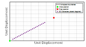Figure 2: Diagonal design with m number of obstacles are alighned diagonally between initial and final locations.

The relationship between the diagonal obstacles and the average successful steps for every m diagonal obstacles are computed and plotted in Figure 3. The results show that the more linear obstacles are added between the start and final positions, the less steps will require AGV to find the desired location.

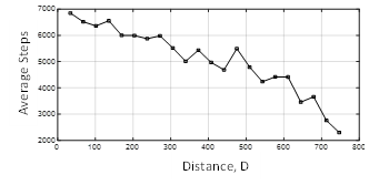Figure 3:  The effect of installing diagonal obstacles on the success of a ranging AGV to finds its destination.

The probability of occurrence, i.e. the long-term probability in equation (2), is simulated for workspace area of size (20 20) unit square with eight obstacles located between initial point (1,1) unit, and final point (10,10) unit. The probability of occurrence can help predict the robot path and warn the facility workers about which area to avoid during work. It can be easily concluded from the results in Figure 4 that the probability of occurrence of robot colliding with nearby obstacle increases. In addition, the chance to find the AGV elsewhere in the workspace is uniformly minimum. As a result, an AGV exhibiting a random walk in a confined area can find its destination faster by creating a physical or virtual diagonal obstacle within proximity of desired final location. In general, one advantage of installing the obstacle is due to the high probability of finding a robot nearby the boundary.

Figure 4: Probability of occurrence for the diagonal obstacle design.

7.2. L-Shape Obstacle Design

The second case study deals with an obstacle design configured in L-shape with fixed width, W, as suggested in Figure 5. The length of the L-shape corresponds to the maximum linear distance traveled between two points within the workspace. The initial and final desired position of a free ranging AGV are assumed at (1,1) and , respectively. The AGV stays within the L-shape area. Algorithm (1) is executed to determine the average number of successful steps for various width.

Figure 5: Example of ‘L- shaped’ obstacle containining the initial and desired locations.

Multiple simulations are carried out for widths ranging from  and at step size, , of one unit. Consider three set of workspaces sizes (50 50), (75 75) and (100 100) unit square. The average success vs. width of L-shape is computed for workspace size, and all curves are plotted in Figure 6.a. Let the “efficiency” be defined by the average success normalized to the area size of the workspace. The average steps/enclosed L-shaped obstacle area is plotted in Figure 6.b.

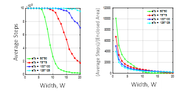Figure 6: L-shape obstacle design.: (a) Success simulated for several widths and workspaces sizes. (b) Effeciency of successful search.

Let a cutoff threshold of 10⁵ define the maximum number of steps before the AGV stops searching. Figure 6.a shows a rapid decay relationship, where it takes an AGV less steps to succeed in smaller workspace. The normalized plot in Figure 6.b implies that the exponential decay relationship becomes independent of the workspace size when the width size is large. However, the overall efficiency of search is better for the large workspace size within W [1 ~7] unit.

7.3. Passage Obstacle Design

Passage obstacle design refers to rectangular area that confines the movement of AG, as suggested in Figure 7. It is assumed that the starting and final positions are always located within the passage area, and distance between these points defines the passage length. In this case study, the intent is to determine how the width of the passage, W, relates to the success of the AGV to find final position. Let the starting and final position be at (1,1) unit, and (a-1, b-1) unit, respectively. Algorithm (1) is deployed to study this relationship for various workspaces sizes, including (50 50), (75 75), (100 100), and (125 125) unit square. The simulation is also carried out for width unit, and at step size, , of 1 unit. It can be observed from the results shown in Figure 8.a that the size of the workspace has little significance to the average success. The average success drops significanly for widths ranging from 1 to 5 unit. This sharp exponential decay could explain why all workspaces have almost identical efficiency, as observed in Figure 8.b.

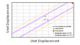Figure 7: Passage Design is created encompassing the initial and desired location of AGV.

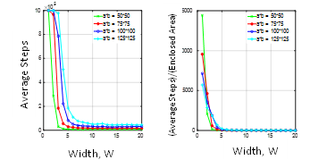Figure 8: Passage obstacle design: (a) Success simulated for several widths and workspaces sizes. (b) Effeciency of successful search.

A more in-depth simulation is performed to examine if the curves in Figure 8.a reach steady state. To make the analysis more robust, a higher walk value of 9600 is chosen, as it is highly likely to converge to the true value. Across different workspace sizes, it is observed that the average steps concave up after attaining its lowest possible value. It is evident from Figure 9 that the lowest value corresponds to an optimum width at which the average number of steps is minimum. It is, however, important to note that the increase in the optimum width is very small with respect to the increase in workspace sizes. It is also observed that the optimal width shifts up as workspace size increases.

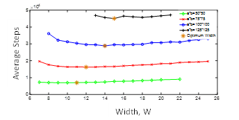Figure 9: Optimum widths for passage design computed at different workspace sizes.

7.4. Defected Passage Obstacle Design

Consider p number of consecutive obstacles being removed from the passage design. Let the defects be present in the “lower side” or “upper side” of the passage as shown in Figure 10. These two configurations are asymmetric along the diagonal line that connects the initial to final position. However, the large area that is open to the passage is equivalent in both case, and therefore, simulations will be carried out separately for each case.

Figure 10: Example of defect on one diagonal side of the passage: (a) Lower side defect (b) Upper side defect.

Figure 11: AGV success in the realm of defective obstacle design.

The simulations are carried out for “upper side” and “lower side” defected passage within the workspace of ) unit square. The goal is to plot the average success against the number of obstacles removed. The order of the obstacle removed in the “lower side” case is chosen to begin from the lower corner of the workspace, i.e. removal begins closer to the initial position. The “upper side” case, however, begins from the upper corner of the workspace, i.e. removal begins from the final position. The maximum number of obstacles in each side is 28 units. It is clear from the simulation results in Figure 11 that in the case of defects in the “lower side”, the average success improves (or linearly decreasing) as the defects (or the number of sequentially removed obstacles) increase. Whereas an exactly opposite effect is observed for the defect in the “upper side”. The slopes obtained from the linear regression for defects [1 27] are equal in magnitude, but opposite as observed in Figure 11. This implies that when k=1, the average success is identical whether the obstacle is removed from upper side or lower side. However, the average success is farthest apart when only one obstacle is left close to the “upper side” or “lower side”. Interestingly, placing only one obstacle near to the final position would significantly improve the success of the AGV to find its final position. However, at p=28, the average steps between lower and upper sides drops drastically and becomes identical simply because the entire obstacles in the diagonal side is removed.

7.5. Zig-zag Obstacle Design

Zig-zig obstacle, such as example in Figure 12, could be utilized across the workspace to mimic certain complexities of an industrial workspace. The average success of an AGV performing SRW is studied against widths by using Algorithm (1). The width, W, defined in Figure 12, is varied between  unit, with increment, of 1 unit. Various workspaces sizes were tested including (50 50), (75 75), (100 100), and (125 125) unit square.

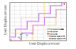Figure 12: Example of zigzag obstacle design.

The simulation result shown in Figure 13.a depicts a fluctuating decay of the average success as the width increase. In addition, the average success curves, corresponding to each workplace size, are significantly spread apart from each other. These effects could be related to irregularity of the obstacle design, especially because the interior search area is sensitive to the width. On the other hand, the normalized plot in Figure 13.b shows that the efficiency of search in the zigzag design is approximately uniform when the workspace size is scaled.

Figure 13: Zig-zag obstacle design: (a) The average success is simulated for several widths and workspaces sizes. (b) Effeciency of successful search.

7.6. Comparison Between Obstacle Designs

A simulation study is conducted to evaluate how effective the obstacle designs are, in terms of their ability to guide an AGV from initial position (1,1) into a final desired position located at . Consider the test conducted on a workspace size of (50 50) unit square. The average success is simulated for passage, L-shaped and zigzag designs, and for various width. The results shown in Figure 14 shows that the passage design performed better than other types for all simulated widths. The L-shape obstacle design was the least effective, however, the decay profile is smooth, and it could be approximated by Cosine Annealing function.

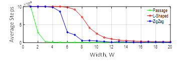Figure 14: Comparison between passage, L-shaped and zigzag design.

8. Simulation: Randomly Walking AGV within Random Static Obstacles and in Confined Workspace

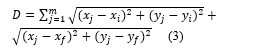
A case study is put forward to examine the relation between a free ranging AGV, and m number of random obstacles placed inside a workspace. Let the degree of obstacle aggregation be defined by scattered distance

where  is the mean value of the scattered obstacles. Simulations are carried out to calculate the average success for m number of various subsets of randomly placed obstacles. Each m subset of obstacle was also iterated, q, number of times.

A simulation example is conducted for an AGV roaming within a confined workspace area of (50 50). The AGV is assumed to be initially placed at (1,1) unit, with target destination located at (25,25) unit. Consider that m subsets belong to individual values in set {1,4, 9,16, 25, 36}. The number of iterations tested per subset is set to q=50. The average success is plotted against the scattered distance and linear accumulative distance (Equation 3) for every iteration, with results shown in Figure 15.

Let the dispersion of randomly placed obstacles, ?, be defined by the range of  for q iterations of a subset m. Also, let the variation in the average success, ?, be defined by the range of the average successes obtained for q iterations of a subset m. The following observation can be depicted from Figure 15.a: (1) Although the average success computed for each iteration seems random, the mean-value calculated for all the average success iterations increases as m increases, i.e. has a negative impact, and (2) ? and ? widen as m increases. The linear cumulative indicator, D, used in the simulation shown in Figure 15.b, references the obstacles relative to the initial and final positions, instead of the mean-value. The difference between D and D_s indicators is regarded to the dispersion of data points. The D value of each m obstacles correspond to distinct aggregation as compared to D_s.

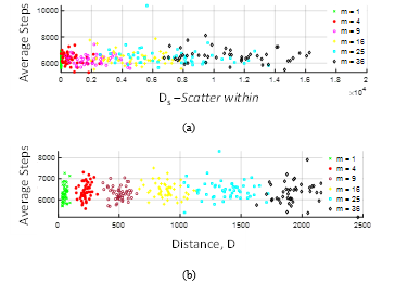Figure 15: The effect of randomly placed static obstacles on the success of a free ranging AGV to find its destination .(a) compared with scattered distance. (b) compared with linear accumulative distance.

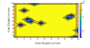Figure 16: Probability of occurance  for randomly placed static obstacles.

An example of long-term probability is simulated for an AGV performing random walk in a workspace (20 20) unit square, amidst 10 randomly generated static obstacles. Figure 16 shows long-term likelihood of the AGV to be present in the light region, “yellow-color”, whereas the dark regions, “blue-color”, corresponds to avoided region.

9. Simulation: Multiple Randomly Walking AGVs in Confined Workspace

This study mimics a real-world collaborative workspace where human-robot or robot-robot interactions co-exist in a confined workspace with randomly placed static obstacles. Mobile robots or AGVs, and human motion are assumed to undergo independent SRW.

The first simulation case study is based on AGV performing SRW motion from the initial point to the final point in the presence of another independent AGV that is in 5-state Markov Chain motion. The Markov Chain implies that the AGV can only jump from one state into one of the other 5-states located within the workspace. Let the workspace size be assigned to (50 50) unit square, with the initial and final desired position for one AGV be located at point unit, and   unit, respectively. Algorithm (2) is implemented to compute the average number of successful steps and the average collision probability by using 300 random walks per test.

Figure 17: Simulation of collision probability of an AGV and a ‘5 state Markov Chain’ AGV, in workspace free of obstacles.

The simulation calculates the average success against the collision probability for 150 random tests, with results shown in the scatter plot in Figure 17. The linear regression fit has a slight negative slope; indicating that an increase in the probability of the collision between the two AGVs has resulted in a decrease in the average success of the free ranging AGV. The mean values of the scatter plot data are approximately, ~ , which is uniquely characterizes the average number of successful steps and probability of collision for the given boundary conditions.

The second case study considers (m+1) independent AGVs in dynamic motion, where all are assumed to undergo simple random walk, i.e. they can travel from any point to another point in a step wise manner. One of these AGVs is tasked to navigate from same the previous initial to the final desired positions, while others are in continuous random motion. The obstacle avoidance is enforced between any combination of AGVs, while all are kept inside workspace. Conversely, this case study is equivalent to a robot swarming among a crowd of randomly moving humans.

Figure 18: Collision Probability of an AGV performing SRW with ‘m’ number of SRW AGVs.

Simulations are carried out for several number of AGVs described in group set m= {1, 2, 3, 4, 5}, where each group is simulated 50 iterations.  The scattered data shown in Figure 18 indicates that the mean values of the average steps evaluated for each group are approximately equal.  I.e., the number of roaming AGVs, m, has little impact on the average success. However, the increase of number of AGVs installation results in increase in the probability of collision.

The effect of the diagonal distance measured between the initial and final positions, R, is examined within the context of this case study. Let the workspace be modified into (100,100).  The average success is simulated for same set of groups and plot against R. This relationship is linear for all m, as shown in Figure 19.

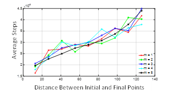Figure 19: The effect of distance between initial and final points on the success of a free ranging AGV to finds its destination.

In addition, the linear plots confirm that in an industrial workspace, increasing random dynamic obstacles has no impact on the average number of steps required for an AGV to find its destination.

10. Conclusions

This paper examined the random walk locomotion in confined workspace.  The goal of the research is to help design a safe shared workspace where humans and robots could co-exist, and further propose a navigation-free method that could help AGVs with malfunctioned navigation retrieve to a safe location at worse case scenarios. The research tested the hypothesis that placing obstacles in workspace could improve the ability of AGV to locate its destination. Several patterns were tested including L-shape, passage, and zigzag. In general, it can be concluded that as the area (characterized here by the width) of obstacle region increases, the AGV will take greater number of steps to reach its final position. However, there exist a threshold at which the increase of the width would have no effect. Passage Design’ is the most efficient way to guide AGV to its final position. In the case of dynamic obstacles, if the obstacles are in Markov chain, the lost AGV will reach its final position in a minimum average number of steps. Finally, as the number of randomly placed obstacles increases, the average number of steps taken by the AGV to reach its final position increases.

11. Future Work

Future work will extend the 2D random walk to study 3D complex interaction of swarm of robots based on Brownian motion model.

Acknowledgement

This study was funded by Ohio Department of Higher Education (ODHE) and Regionally Aligned Priorities in Delivering Skills Program (RAPIDS 4.0) grant “Automated Guided Vehicles for Smart-logistics and Safe Material Handling in Advanced Manufacturing and Warehouse Industries.

Conflict of Interest

The authors declare that they have no conflict of interest.

1. R. Bostelman, “AGMs and forklifts gaining sight for safety,” Material. Handling and Logistics Magazine., 68(1), 34–37, 2013, https://tsapps.nist.gov/publication/get_pdf.cfm?pub_id=912983.
2. SICKUSAblog, “Additional solutions for collision avoidance with indoor AGVs,” SICKUSAblog, https://sickusablog.com/additional-solutions-collision-avoidance-indoor-agvs/, Jul. 2019.
3. R. Koster, T. Le-Anh, J. van der Meer, “Testing and classifying vehicle dispatching rules in three real-world settings,” Journal of Operations. Management, 22(4), 369–386, 2004, https://doi.org/10.1016/j.jom.2004.05.006.
4. A. P. Vancea, I. Orha, “A survey in the design and control of automated guided vehicle systems,” Carpathian Journal of Electronic and Computer Engineering, 12(2), 41–49, 2020, doi: 10.2478/cjece-2019-0016.
5. E. Cardarelli, L. Sabattini, V. Digani, C. Secchi, C. Fantuzzi, “Interacting with a multi AGV system,” in IEEE Intelligent Computer Communication and Processing International Conference, 263–267, 2015, doi: 10.1109/ICCP.2015.7312641.
6. A. Prusak, J. Bernshausen, H. Roth, J. Warburg, C. Hille, H.-H. Gtting, T. Neugebauer, “Applications of automated guided vehicle (AGV) and industry robots with PMD-camera,” 2007, 299-303.
7. C. Liu, M. Tomizuka, Designing the robot behavior for safe human–robot interactions, Springer Internatinoal Publishing, 2017.
8. L. Sabattini., V. Digani, C. Secchi, G. Cotena, D. Ronzoni, M. Foppoli, F. Oleari. “Technological roadmap to boost the introduction of AGVs in industrial applications,” In 2013 IEEE 9th International Conference on Intelligent Computer Communication and Processing 203–208, 2013, doi: 10.1109/ICCP.2013.6646109.
9. B. S. P. Reddy & C. S. P. Rao, “A hybrid multi-objective GA for simultaneous scheduling of machines and AGVs in FMS,” Internatinal Journal Advanced Manufacturing Technology., 31, 602–613, 2006, doi: https://doi.org/10.1007/s00170-005-0223-6.
10. M. V. S. Kumar, R. Janardhana, and C. S. P. Rao, “Simultaneous scheduling of machines and vehicles in an FMS environment with alternative routing,” Internatinal Journal Advanced Manufacturing Technology, 53(1-4), 339–351, 2011, doi: 10.1007/s00170-010-2820-2.
11. J. Jerald, P. Asokan, G. Prabaharan, and R. Saravanan, “Scheduling optimisation of flexible manufacturing systems using particle swarm optimisation algorithm,” Internatinal Journal Advanced Manufacturing Technology, 25(9–10), 964–971, 2005, doi: 10.1007/s00170-003-1933-2.
12. N. Krishnamurthy, R. Batta, M. Karwan, “Developing conflict-free routes for automated guided vehicles,” Operations Research, 41(6), 1077–1090, 2018, https://doi.org/10.1287/opre.41.6.1077.
13. D. Zeitler, M. Werner, G. Koff, “Dynamic object avoidance with automated guided vehicle”, Washington, DC, US Patent 20050021195, 2005.
14. D. Emanuel, R. Kunzig, R. Taylor “Method and apparatus for collision avoidance” Washington, DC, US Patent 8346468B2, 2013.
15. T. Park, “AGV control system and method,” Washington, DC, US Patent 7305287B2, 2007.
16. J. Kondo, “Travel control device for unmanned conveyence vehicle,”, Washington, DC, US Patent 8406949B2, 2013.
17. S. Lee, W. Jeong, “Apparatus and method for estimating a position and an orientation of a mobile robot” Washington, DC, US Patent, 20100070125A1 2010.
18. P. Lasota, T. Fong, J. A. Shah, “A Survey of methods for safe human-robot interaction,” Foundation and Trends in Robotics., 5(3), 261–349, 2017, doi: 10.1561/2300000052.
19. G. Michalos, S. Makris, P. Tsarouchi, T. Guasch, D. Kontovrakis, G. Chryssolouris, “Design considerations for safe human-robot collaborative workplaces,” Procedia CIRP, 37, 248–253, 2015, doi: 10.1016/j.procir.2015.08.014.
20. R. Inam, K. Raizer, A. Hata, R. Souza, E. Forsman, E. Cao, S. Wang, “Risk Assessment for human-robot collaboration in an automated warehouse scenario,” in 2018 IEEE 23rd International Conference on Emerging Technologies and Factory Automation (ETFA), 743–751, 2018, doi: 10.1109/ETFA.2018.8502466.
21. E. Magrini, F. Ferraguti, A. Ronga, F. Pini, A. De Luca, F. Leali, “Human-robot coexistence and interaction in open industrial cells,” Robotics Computer-Integrated Manufacturing, 61, 101846, 2020, doi: 10.1016/j.rcim.2019.101846.
22. I. Draganjac, D. Miklic, Z. Kovacic, G. Vasiljevic, S. Bogdan, “Decentralized control of multi-AGV systems in autonomous warehousing Applications,” Transactions on Automation Science Engineering, 13(4), 433–1447, 2016, doi: 10.1109/TASE.2016.2603781.
23. R. Miller, R. Subrin, Automated Guided Vehicles and Automated Manufacturing. Society of Manufacturing Engineers, 1987.
24. N. Möller, S. Ove Hansson, J. Holmberg, C. Rollenhagen, Handbook of Safety Principles, Wiley, 2018.
25. T. Helmer, Development of a methodology for the evaluation of active safety using the example of preventive pedestrian protection, Springer Internatinoal Publishing, 2015.
26. MMH Staff, “AGVs enhance automotive powertrain production,” Modern Material Handling, Oct. 2018.
27. AGV Technology, “Understanding AGV safety systems,” AGV Network, https://www.agvnetwork.com/automated-guided-vehicles-safety-systems, Jun. 2020.
28. C Frese, A Fetzner, C. Frey. “Multi-sensor obstacle tracking for safe human-robot interaction”, in International Symposium on Robotics, 784-791, 2014, permalink http://publica.fraunhofer.de/documents/N-298607.html.
29. J. H. Chen and K. T. Song, “Collision-free motion planning for human-robot collaborative safety under cartesian constraint,” in 2018 IEEE International Conference on Robotics and Automation (ICRA), 4348-4354, 2018, doi: 10.1109/ICRA.2018.8460185.
30. P. Wenger, P. Chedmail, “Ability of a robot to travel through its free work space in an environment with obstacles,” International Journal of Robotics Research, 10(3), 214–227, 1991, doi: 10.1177/027836499101000303.
31. N. Vahrenkamp, H. Arnst, M. Wachter, D. Schiebener, P. Sotiropoulos, M. Kowalik, & T. Asfour. “Workspace analysis for planning human-robot interaction tasks,” in 2016 IEEE-RAS 16th International Conference on Humanoid Robots, 1298–1303, 2016, doi: 10.1109/HUMANOIDS.2016.7803437.
32. F. Rezazadegan, J. Geng, M. Ghirardi, G. Menga, G. Camuncoli, “Risked-based design for the physical human-robot interaction ( pHRI ): an overview,” Chemical Engineering Transactions, 43, 1249–1254, 2015, doi: 10.3303/CET1543209.
33. E. Kim, R. Kirschner, Y. Yamada, S. Okamoto, “Estimating probability of human hand intrusion for speed and separation monitoring using interference theory,” Robotics and Computer-Integrated Manufacturing., 61, 101819, 2020, doi: 10.1016/j.rcim.2019.101819.
34. A. Lambert, D. Gruyer, G. Saint Pierre, “A fast Monte Carlo algorithm for collision probability estimation,” in 2008 10th International Conference on Control, Automation, Robotics and Vision, 406-411, 2008, doi: 10.1109/ICARCV.2008.4795553.
35. J. van den Berg, P. Abbee, K. Goldberg, “LQG-MP: Optimized path planning for robots with motion uncertainty and imperfect state information,” International Journal of Robotics Research, 30(7), 895–913, 2011, doi: 10.1177/0278364911406562.
36. S. Patil, J. van den Berg, R. Alterovitz, “Estimating probability of collision for safe motion planning under Gaussian motion and sensing uncertainty,” in IEEE International Conference on Robotics and Automation, 3238-3244, 2012, doi: 10.1109/ICRA.2012.6224727.
37. F. Flacco, T. Kroeger, A. De Luca, O. Khatib, “A depth dpace approach to human-robot collision avoidance,” in 2012 IEEE International Conference on Robotics and Automation (IRCA 2012), 338 – 345, 2012, http://toc.proceedings.com/15154webtoc.pdf.
38. J. H. Liang, C. H. Lee, “Efficient collision-free path-planning of multiple mobile robots system using efficient artificial bee colony algorithm,” Advances in Engineering Software, 79, 47–56, 2015, doi: 10.1016/j.advengsoft.2014.09.006.
39. N. Pedrocchi, F. Vicentini, M. Malosio, L. M. Tosatti, “Safe human-robot cooperation in an industrial environment,” International Journal of Advanced Robotic Systems, 10(1), 2013, doi: 10.5772/53939.
40. M. Mayyas, S. P. Vadlamudi, M. A. Syed, “Fenceless obstacle avoidance method for efficient and safe human–robot collaboration in a shared work space,” International Journal of Advanced Robotic Systems, 17(5), 2020, doi:10.1177/1729881420959018.
41. D. Claes, K. Tuyls, “Multi robot collision avoidance in a shared workspace,” Autonomous Robots, 42(8), 1749–1770, 2018, doi: 10.1007/s10514-018-9726-5.
42. C. Park, J. Park, D. Manocha, “Fast and bounded probabilistic collision detection for High-DOF trajectory planning in dynamic environments,” Transactions on Automation Science and Engineering, 15(3), 980-991, 2018, doi: 10.1109/TASE.2018.2801279.
43. J. H. Cho, D. S. Pae, M. T. Lim, T. K. Kang, “A Real-Time Obstacle Avoidance Method for Autonomous Vehicles Using an Obstacle-Dependent Gaussian Potential Field,” Journal of Advanced Transportation, 2018, 2018, 5041401, doi: 10.1155/2018/5041401.
44. S. Carpin, G. Pillonetto, “Motion planning using adaptive random walks,” IEEE Transactions on Robots., 21(1), 129–136, 2005, doi: 10.1109/TRO.2004.833790.
45. L. Palmieri, A. Rudenko, and K. O. Arras, “A fast random walk approach to find diverse paths for robot navigation,” IEEE Robotics and Automation, 2(1), 269–276, 2017, doi: 10.1109/LRA.2016.2602240.
46. B. Pang, Y. Song, C. Zhang, H. Wang, R. Yang, “A swarm robotic exploration strategy based on an improved random walk method,” Journal of Robotics, 2019, 2019, doi: 10.1155/2019/6914212.
47. M. Biskup, Random walks. 1827.
48. A. Singh, “Reinforcement learning?: Markov-decision process (Part 1),” 2019, https://towardsdatascience.com/introduction-to-reinforcement-learning-markov-decision-process-44c533ebf8da.
49. E. Behrends, Introduction to Markov chains, Friedr. Vieweg & Sohn Verlagsgesellschaft mbH, 2000.
50. Ryan O’Donnell, Great Ideas in theoretical computer science: Random walks and Markov chains [Video] You Tube, July 15, 2017 https://www.youtube.com/watch?v=86N-awvgi1w, 1:19:31.
51. N. Etemadi, “An elementary proof of the strong law of large numbers,” Zeitschrift für Wahrscheinlichkeitstheorie und Verwandte Gebiete, 55, 119–122, 1981, doi: 10.1007/BF01013465.

(Click Here)