1. Introduction

This paper is an extension of the work originally presented in ICARA [1]. Further investigations to increase performance of the approach are done changing deep learning parameters, moreover problem simplification and data augmentation have been tested.

The field of the proposed paper is navigation system and related localization, which is still considered a challenging task [2]. The core function of these kind of systems is for sure the localization itself. Main goal of this vital function is the correct estimation of the step-by-step position of the moving robot in unknown scenes. To perform this task different data sensors can be used. Moreover, to reach better estimation usually previous step data are stored inside an updating map.

About localization approaches proposed in literature, two main localization groups can be recognized: vision-based and laser-based.

Vision-based localization techniques just use images to achieve their goal. Usually, features inside previous and current image are calculated and matched to retrieve the global displacement. In literature, different vision-based techniques have been proposed:  effective prioritized matching [3], ORB-SLAM [4], monocular semi-direct visual odometry (SVO) [5], camera pose voting [6], localization based on probabilistic feature map [7], etc. More sophisticated solutions, like multi-resolution image pyramid methods, have been proposed to reach more robust feature matching [8]. These approaches are usually robust, but they do not have useful distance information, i.e., it is difficult to map the estimated trajectory (in pixel) in the real world (in cm).

On the other hand, laser-based localization techniques just use laser scans to achieve their goal. A features matching approach, as in vision-based localization, is not simple to be implemented. This is mainly due to the poor information of laser scans compared to images. In fact, in the case of image details (e.g., corners), we can note only weak variations in range measurements and then a lack of distinctive features to be analyzed [9].

Usually, Bayesian filtering are largely used in laser-based techniques to consider the robot position as a problem of probability distribution estimation based on grid maps [10,11]. Apart Bayesian filtering, in literature other laser-based proposed techniques are: iterative closest point (ICP) [12] and related variants [13], which minimize the matching error between two point-clouds estimating the related transformation, perimeter based polar scan matching (PB PSM), Lidar odometry and mapping (LOAM) [15], which achieves real time processing by running in parallel two different algorithms, and so on. Even if these approaches usually achieve precise localization, since distance information is available, they can fail in scene changing conditions. In fact, when an object is moving in the scene, due to the occlusions, we can have lack of information in the moving object area and then the estimated localization can be wrong.

Recently, in vision-based localization, to extract and match image features, deep learning approaches have been successfully used. These promising approaches allow to estimate camera position. A lot of deep learning approaches have been proposed in literature: PoseNet [16], which for pose regression task uses the convolutional neural networks (CNNs), Deepvo [17], which for the same task uses recurrent neural networks (RNNs), undeepVO [18], which estimates the monocular camera pose using a deep learning unsupervised method, and so on. Unfortunately, at moment the deep learning-based methods do not achieve the same pose estimation accuracy of classical vision-based localization approaches.

Inspired by vision-based localization approaches based on deep learning algorithms, few attempts of deep learning methods have also been suggested for laser-based localization: in [19] authors estimate odometry processing 3D laser scanner data with a series of CNNs, in [20] authors trained for giving steering commands a navigation model target-oriented, in [21] authors performed loop closure and matching of consecutive scans making use of a CNN network, in [22] authors improved the odometry estimation considering also temporal features using a RNN, able to model sequential long-term dependencies, and so on.

Regarding the deep learning laser-based localization, as indicated in the case of vision-based localization, unfortunately they still do not achieve the accuracy of the pose estimation compared to classical laser-based localization. For this reason, in literature some authors propose the integration of deep learning approaches with the classical ones: in [23] the authors make use of Inertial Measurement Unit (IMU) in combination with CNNs for 3D laser scanners for assisted odometry, in [24] the authors use the result of vision-based localization approaches based on CNN as starting seed for Monte Carlo localization algorithm, to speed-up algorithm convergence, also increasing robustness and precision, and so on.

It is easy to understand that the field of deep learning localization, in particular about laser-based approaches, has not yet been intensively explored and, at moment, it is still considered a challenging process. In fact, just a small number of papers discuss about this subject [22]. Our choise is to go further in this investigation, to obtain a simple deep learning laser-based localization, using only data taken by 2D laser scanners. Moreover, we tried to reduce as far as possible the number of parameters used by the proposed network, to deal with the low-cost resources constraint.

Our contribution to the research in the field of navigation system, using deep learning approaches, with only 2D laser scan input is firstly the exploration of state of art algorithms. Another contribution is to indicate a methodology to generate the ground truth for the neural network without using real sensors but simulating them with existing powerful navigation tools.

Novelties of the proposed system are in both neural network dataset generation and training. In particular, in data generation we indicate a methodology to choose properly the angle resolution trying to reduce the collisions per frame (to avoid loss of important data) and to maximize array density (to avoid working with sparse data). In this way, the neural network was more able to solve the regression problem.

In the training phase, the novelty is the demonstration with real tests that in regression problems the choice of input/output values scale is vital to let the neural network working. In fact, after several experiments,  we obtained the correct scale measures for distances and angles.

At last, the great contribution was to find, after lots of experiments with various neural network hyper parameters, a really light network to solve the localization problem with good performances in terms of  mean absolute error between estimated positions and ground truth.

The proposed research is composed by the following Sections: Section 2, where the proposed deep learning laser-based localization is described; Section 3, where the experimental results obtained are deeply described; Section 4, where final considerations are remarked.

2. Proposed Approach

A typical navigation system is described in Figure 1. A starting moving object position (x,y,α) is considered, where (x,y) are the horizontal and vertical position in the cartesian axis and α is the orientation angle. Usually, at the beginning the position is assumed to be (0,0,0). Every time laser scan data is available (θ, d), where  θ is the angle and d is the distance from object in front of the laser beam, the localization step will calculate the new position (x’,y’,α’). The system will then decide next movement. Depending on how it is programmed the moving object (for example the robot), the system can decide to continue moving (in the case an obstacle is not found) or to stop motors (when an obstacle is found). The correct command are then send to the motor control (which interact with the IMU) to update the movement. Positions and movements are updated each time.

Inside the navigation system, the proposed deep learning approach is applied on the core localization step. From this point, this article will focus only on the localization step and all the research will be focused on this particular block of the navigation system.

To reach this objective we used a wheeled robot equipped with the laser scanner A2 RPLidar on the top. This rotating laser scanner has twelve meters as maximum range, view at 360 degrees, running up to fifteen Hz. Thanks to the robot, we acquired a custom dataset in various environments (apartment, laboratory and office).

The ground truth generation schema used is shown in Figure 2. At the beginning, the dataset acquisition is needed to record the input Lidar dataset. Each scan is composed by multiple couples (d, θ), where d is the distance from the object and θ is the related angle. Once the dataset was obtained, we needed to generate the ground truth position (x, y, α) for each sample taken. Since we do not have the real position of the robot for each scan contained in the acquired dataset, we needed a simulation environment to obtain a ground truth.

For this purpose, we make usage of the MATLAB Navigation Tool. The generated ground truth was tested using a simple Mat2Map program to display the path of obtained positions (x, y, α) for each sample taken and the map generated by Lidar scans. In this way, we also checked the robustness of  Navigation Tool. Even if it is a very slow method, we tested it in different conditions and we conclude to be very precise, so it was used as reference.  It is based on Google Cartographer [25], which builds multiple submaps and try to align upcoming scans with previous nearby submaps, generating the constrains on a graph.

Once we generated the custom dataset and related ground truth, we perform our experiments using the TensorFlow framework with Keras wrapper in a Python environment. In this configuration, to obtain the best compromise between quality and complexity, we tried different data binarization and augmentation with various neural network configurations.

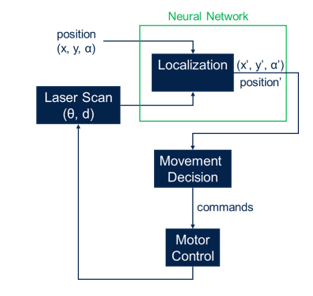Figure 1: Navigation system.

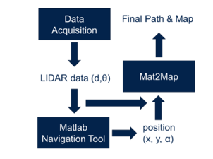Figure 2: Ground truth generation schema.

2.1. Dataset Generation

The main challenge in deep learning approaches is the acquisition of large amounts of data, to allow the neural network to work fine in any real scenario. Our generated dataset consists in about 51,000 samples, which we tested to be enough in our experiments for training the proposed neural network. Each sample is composed by two subsequent scans acquired by Lidar. Each scan is expressed by multiple couples (d, θ), that is the distance and the angle from the nearest found object.

Data acquisition cannot be used as it is.  We instead need to encode acquired data into a panoramic like depth image, so we need a sort of binarization of each scan before to be paired with the following one. Data binarization is inspired by a previous work [21] to encode laser scans into a 1D vector. To obtain a 1D vector, in each scan, all distances are binned into angle bins, according to the chosen angle resolution. In this way, we stored all depth values inside a 1D vector, where all the possible depths are represented (from 0° to 360°). As soon as two subsequent scans are binarized, we can couple them to be used as neural network input.

Laser range scanners usually give (scan by scan) distances from the identified nearest object for constant angles, so binarization is simple, because we have a fixed number of possible angles to be considered into the 1D vector. Instead, in the chosen laser range scanner A2 RPLidar in each scan the angles can vary, from 0° to 360°. For this reason, it is not possible to fix we the angle resolution as in previous works, e.g., in [22] the authors use 0.10° and in [21] the authors use 0.25°, so a preliminary investigation to find optimal angle resolution is needed. In this research, we tried at the same time to maximize array density and to minimize collisions per frame. Array density is for each scan the number of non-zero value bins, while collisions per frame is the total number of data ranges which are in the same bin.

Table 1 shows the impact of the chosen β (angle resolution) on N (total number of bins) and then on mean collisions per frame and mean array density. Since A2 RPLidar have got a 360 degrees view, the laser data is separated into β degree bins, for a total amount of N=360°/β° bins. Of course, increasing β (and then decreasing the total number of N bins) the array density increases and of course collisions per frame will become bigger. In our experiments, we tried different angle resolutions β to make at the end the proper decision about which configuration to use in the proposed neural network.

As indicated in Table 1, particularly at higher angle resolutions β, collision is an important aspect to solve to guarantee the neural network to work property. In [22] authors chose to take the mean of all distances are in the same bin, probably because in their experiments the collision occurred rarely and distances at the same degree was similar. In our experiments, we consider two main aspects: laser range scanner is more precise for lower distances and average of two different distances at the same degree can introduce false objects distances. For these reasons, we choose to take the minimum distance (instead of average distance) for distances falling in the same degree.

Table 1: Dataset Binarization

β	N	Collisions per frame	Array Density
0.10	3600	0.05	9%
0.25	1440	0.13	22%
0.50	720	0.48	46%
1.0	360	2.54	89%

2.2. Neural Network

The network we propose in this work, from a consecutive pair of two scans (s_t-1,s_t) done by the chosen Lidar, obtains the robot displacement between them, trying the estimation of their relative pose transformation:

where Δx and Δy are respectively the horizontal and vertical translations and Δα is the rotation angle between the two scans (s_t-1,s_t). We can only estimate the displacement of the robot in two dimensions, since we choose to use just a two dimension sensor.

The final objective of the neural network is to learn the unknown function g(), which, at time t, maps (s_t-1,s_t) to the pose transformation T :

In the training step the unknown function g() is learned. Moreover, thanks to the accumulation of the estimated local poses from the starting of the process up to time t, we obtain the robot global position at time t. The chosen loss functions are: mean absolute error (MAE) and mean square error (MSE), which are commonly used in deep learning regression problems.

The strategy we tried to implement here is to fit our regression problem with standard deep learning 2D image matching problems. The difference is that, in our case, instead of 2D images, we have obtained (thanks to dataset binarization) 1D panoramic depth images. In this way, as in the case of images, we can use consecutive CNN to extract spatial features obtained by the sensor in the tested conditions. After that, additional fully connected layers (dense layers) allow to the neural network to understand patterns within extracted spatial features to provide the matching and then the current robot position estimation in the unknown environment.

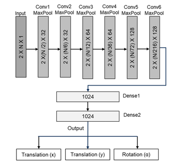Figure 3: Proposed deep learning approach.

Table 2: Parameters of Neural Network

N	NN Model	NN Parameters
3600	CNN+LSTM	21,078,563
3600	CNN+Dense	5,343,779
1440	CNN+LSTM	15,835,683
1440	CNN+Dense	2,722,339
720	CNN+LSTM	14,262,819
720	CNN+Dense	1,935,907
360	CNN+LSTM	13,214,243
360	CNN+Dense	1,411,619

The proposed neural network is shown in Figure 3. The suggested neural network has been inspired by the one indicated in [22], but some differences should be evidenced. Firstly, we make lots of trials to obtain a low complexity neural network, without to lose in quality performance. Moreover, we used max pool layers (instead of average pool layers) reducing complexity and extracting only most important features spatially distributed. Better results were obtained using max pooling, since as aforementioned (see Table 1), the binarized laser scans tends to be sparse, when the angle resolutions β tends to increase. For the same reason, we also eliminate the stride parameter of the various neural network convolutional filters, which can eliminate useful information for sparse binarized laser scans. To maintain the same dimension, instead of using stride parameter in the convolutional filters, we used other max pooling before applying these filters.

As aforementioned, we experimented different neural network configurations, in particular varying:

• β (angle resolution) and then N (number of bins), to define the correct dimension of input data;
• last two network layers, trying both dense layers [21] and long short term memory (LSTM) layers [22].

      The calculation of the NN parameters is shown in Table 2. This number is impacted by N (number of bins) and by the neural network model used. As indicated, when N is increased and when LSTM layers are used, the total number of NN parameters and then the time to be executed will increase too. It is to note that the changes made compared to [22], that is max pool in replacement of strides and average pool, do not impact the overall NN parameters.

2.3. Training

For the sake of clearness, now we indicate in detail the input and ground thru output of the proposed neural network. Input for the network is composed by composed by a set of couples of consecutive Lidar scans (θ, d). These scans are preprocessed allowing to binarize them into sets of 2 X N matrixes, as indicated in Section 2.1. In these matrixes, N depends on β (angle resolution), like indicated in Table 1.

About the reference (ground thru) output of the proposed NN, it is composed by a set of vectors T = [Δx,Δy,Δα], which are the ground thru positions of the moving object, obtained by applying Navigation Tool (MATLAB) to the input Lidar scans (θ, d).

The various experiments were performed in a Python environment with the use of TensorFlow framework and Keras wrapper. Moreover, a workstation was used for training execution, that is a Xeon ES-2630 (Intel) octacore machine with 62 GB of RAM and a Titan X (Pascal) GPU produced by Nvidia. The chosen GPU has got 12 GB of RAM and it is equipped by 3584 CUDA cores, to allow lots of parallelization in training step for faster execution.

The details for training step are the following: 0.0001 function cost minimization learning rate, 500 epochs for training the neural network, 32 batch size and Adam training optimizer used.  We tried other kinds of training optimizers, but we did not notice any significant difference in regression performances.

3. Experimental Results

Lots of tests have been executed with different neural network configurations, as indicated in Table 2, and with different indoor environments. As expected, it is important to note that classical Convolutional Neural Networks (CNNs) work better in the case of dense input datasets. For this reason, we used max pooling instead of average pooling in final tests. For the same reason, even if, at the beginning, we tried in our experiments all the different neural network configurations, final research was focused on β (angle resolution) set to one degree and then N (number of bins) set to 360. This choice also allows us to reduce the total neural network parameters and the overall complexity.

Figures in this Section are representative of a particular testing to underline how (depending on scaling applied) the neural network tends to converge (generalizing the regression problem) or not and to underline how the final suggested neural network fits our needs (lightness and precision). In particular, in the X axis the evolution of the network in various epochs (trials) is represented and in the Y axis the loss in precision is represented (first trials in mean square error, after we used mean absolute error). When train and validation curves are similar with low loss the neural network works properly, while when they are different a problem occurs. In this Section we try to explain a particular reason (scale) of this problem.

Table 3 shows the results obtained using input distances and output positions expressed in millimeters. Results are really bad: the proposed network seems to make a sufficient regression work for training set, but for validation and test set it does not reach good performance at all. In general, as expected, max pooling strategy reaches better performance than average pooling and reducing the angle resolution and then the N dimension of the input binarized scans we obtain better loss values (MSE).

To better understand the evolution of this first experiment done on the proposed neural network epoch by epoch, the first 150 epochs are displayed in Figure 4. This graph is referred to the case N = 1440 with max pooling (train loss = 2.48 MSE; validation loss = 216 MSE; test loss = 233 MSE), but similar considerations can be done on the other different configurations. It is easy to note that while the curve for train decreases, the curve for validation is flat, so the proposed network, in this case, is not able to solve the overexposed regression problem and to generalize it.

Table 3: Test Results (MSE) with Input Dataset (Millimeters)

N	Model	Train Loss	Validation Loss	Test Loss
3600	AvePool	2.78	250	258
3600	MaxPool	2.75	248	250
1440	AvePool	2.30	228	236
1440	MaxPool	2.48	216	233
720	AvePool	2.36	221	240
720	MaxPool	3.27	220	238
360	AvePool	7.54	220	235
360	MaxPool	7.02	218	230

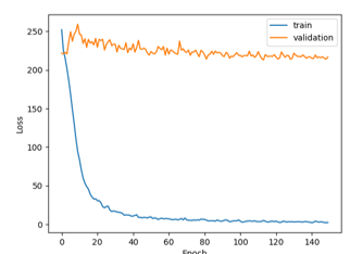Figure 4. Results obtained with input dataset (millimeter).

In the used approach, the main issue is the scale discrepancy in the input variables (x and y expressed in millimeters and α expressed in degree), which often increases the difficulty to correctly model the neural network to solve the regression problem. A common trick used in these cases is to pre-process the input variables before they are fed to the neural network [26]. In the same way, also the outputs of the network (d expressed in millimeters and θ expressed in degree) should be processed to obtain the correct output values.

A commonly used pre-processing step is just a simple linear scaling of network variables [26], so we just changed the distance measure passing from millimeter to centimeter and the related results are shown in Table 4. As indicated, better results are obtained compared to the first tentative with input distances and output positions expressed in millimeters. Even if results are better, we must again to note that they are not good enough: again, the proposed network seems to make a sufficient regression work for training set, but for validation and test set it does not reach similar good performance. Moreover, as expected, max pooling strategy reaches better performance than average pooling and reducing the angle resolution and then the N dimension of the input binarized scans we obtain better loss values (MSE).

Table 4: Test Results (MSE) with Input Dataset (Centimeters)

N	Model	Train Loss	Validation Loss	Test Loss
3600	AvePool	0.09	4.12	3.90
3600	MaxPool	0.03	3.98	3.83
1440	AvePool	0.28	3.97	3.77
1440	MaxPool	0.11	3.87	3.68
720	AvePool	0.18	3.86	3.76
720	MaxPool	0.13	3.84	3.67
360	AvePool	0.28	3.75	3.70
360	MaxPool	0.19	3.67	3.64

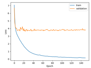Figure 5. Results obtained with input dataset (centimeter).

To better understand the evolution of the second experiment done on the proposed neural network epoch by epoch, the first 150 epochs are displayed in Figure 5. To allow a visual comparison with Figure 4, also this graph is referred to the case N = 1440 with max pooling (train loss = 0.13 MSE; validation loss = 3.84 MSE; test loss = 3.683 MSE). Of course, similar considerations can be done on the other different configurations. It is important  to put into evidence that MSE is not a linear measure, but quadratic. This is the reason why the loss is drastically reduced in comparison with the previous experiment. Moreover, the train curve correctly decreases, as in previous case, while in the current test the validation curve is not completely flat, but it starts to go down. As first experiment, in the current test the proposed network cannot model the neural network to generalize and correctly solve the regression problem, but improvements noticed give us an important hint to work with: to obtain the best regression results, firstly we must find the correct rescaling to apply to input and output data measures (distance and angle).

At this point, we make some rescaling experiments. To maintain similar scale in both input dataset and output variables, we tried to scale translation data by one thousand (in this way we use meters, instead of millimeters as measure) and rotation data by one hundred. This rescaling configuration gives us best results. Furthermore, we decide to make use of Mean Absolute Error (MAE), instead of Mean Squared Error (MSE). In this way, we obtained similar loss curves, but with results simpler to understand and comment, because MAE is a linear measure, while MSE is quadratic. Figure 6 shows that good results are finally reached (train loss: 0.011 MAE; validation loss: 0.011 MAE; test loss: 0.010 MAE), using the new scaling factors to be applied to input and output data with a very simple configuration (only 1,411,619 network parameters). Like other experiments, the train curve correctly decreases, but this time the validation curve also decreases with similar slope. This indicates that finally we reached our main goal: the neural network can now correctly generalize and solve the proposed regression problem.

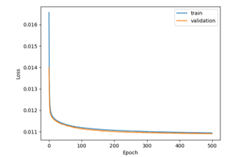Figure 6: Results obtained with input dataset (meter) with 1,411,619 parameters

In our research, we tried to further reduce the parameters in the proposed neural network for lighter solutions, to be implemented in microcontrollers with low resources and in particular with memory (RAM and FLASH). To reach this goal, we tried to reduce the  elements in the last two layers (dense layers). After several trials, we realized that the results are still good also deleting last two layers, obtaining a very low neural network parameters (96,547). Figure 7 shows that in this experiment, even if at the beginning loss values are higher than previous test because the neural network is simpler, at the end of the epochs, train and validation curves are very similar and this network reaches similar results. In fact, Table 5 shows that numerical results between the prosed full neural network with 1,411,619 parameters and the proposed reduced neural network with 96,547 reaches similar performances in terms of MAE regression loss.

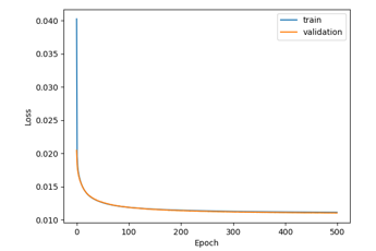Figure 7: Results obtained with input dataset (meter) with 96,547 parameters

Table 5: Test Results (MAE) with Input Dataset (Meters) (N = 360)

P	Model	Train Loss	Validation Loss	Test Loss
1.4M	MaxPool	0.011	0.011	0.010
96K	MaxPool	0.011	0.011	0.010

Table 6: Test Results (MAE) For (x,y) Only (N=360)

P	Model	Train Loss	Validation Loss	Test Loss
1.4M	MaxPool	0.009	0.009	0.010
1.4M	MaxPool Augmentation	0.009	0.009	0.010
96K	MaxPool	0.010	0.010	0.010
96K	MaxPool Augmentation	0.010	0.009	0.009

Further investigations to increase performance of the proposed neural network have also been carried out. In particular, different normalization techniques (scaling) have been tested in our testing environment, like MinMaxScaler() and StandardScaler(), but no substantial improvement has been obtained. The same behavior (no improvement) has been also noticed changing the function loss (Euclidean distance) and extending the neural network using LSTM layers in replacement of Dense layers.

At this point, we tried to reduce the problem limiting the output of the neural network to only spatial components, i.e., to a vector T’ = [Δx,Δy]. Moreover, in this simplified problem version, we also tried an intensive data augmentation, obtained with different strategies. In particular, we take input scans in reverse order, just odds and even scans and finally odds and even scans in reverse order. In this way, we obtained about 204,000 samples, that is about four times the original dataset.

Table 6 summarizes the results obtained by the proposed neural network in the case of simplified problem. Comparing the results with the ones in Table 5, we can note a negligible improvement in train and validation loss, but not in the test loss, so results are almost the same. Even with the intensive augmentation, we obtain a slight but not significant improvement for the simpler neural network with 96,547 parameters.

4. Conclusions

The problem of estimating the moving robot localization, with the only usage of data coming from 2D laser scanner, has been addressed by this paper using a simple deep learning approach. For the dataset used, in the final version composed by 204,000 samples with only 96,547 parameters, the proposed neural network achieved good precision performance in terms of Mean Absolute Error (MAE): one centimeter in translation and one degree in rotation. We also tried to increase performance of the proposed network using different strategies and parameters, but no significant improvements have been obtained.

Even if the encouraging results presented here are almost comparable with classical localization estimation approaches, at moment the approaches based on deep learning could be used in replacement of other state-of-the-art algorithms, since the latter ones are more flexible and can potentially reach better performances. Anyway, the overexposed approach remains a good proof of concept and it can be used for future explorations.

Furthermore, the proposed neural network can be used as interesting complement or can be integrate in classic localization methods, since it works in real-time, taking less than  130 μs to elaborate each estimation on Titan X (Pascal) GPU produced by Nvidia.

Conflict of Interest

None of the authors have any kind of conflict of interest related to the publication of the proposed research.

1. G. Spampinato, A. Bruna, I. Guarneri, D. Giacalone, “Deep Learning Localization with 2D Range Scanner,” International Conference on Automation, Robotics and Applications (ICARA), 206-210, 2021, DOI: 10.1109/ICARA51699.2021.9376424.
2. G. Spampinato, A. Bruna, D. Giacalone, G. Messina, “Low Cost Point to Point Navigation System,” International Conference on Automation, Robotics and Applications (ICARA), 195-199, 2021, DOI: 10.1109/ICARA51699.2021.9376545.
3. T. Sattler, B. Leibe, L. Kobbelt, “Efficient & Effective Prioritized Matching for Large-Scale Image-Based Localization,” IEEE Transaction on Pattern Analysis and Machine Intelligence, 1744-1756, 2017, DOI: 10.1109/TPAMI.2016.2611662.
4. R. Mur-Artal, J. M. M. Montiel, J. D. Tardos, “ORB-SLAM: a versatile and accurate monocular SLAM system,” IEEE Transactions on Robotics, 31(5), 1147-1163, 2015, DOI: 10.1109/TRO.2015.2463671.
5. C. Forster, M. Pizzoli, D. Scaramuzza. “SVO: Fast semi-direct monocular visual odometry,” IEEE International Conference on Robotics and Automation (ICRA), 15-22, 2014, DOI: 10.1109/ICRA.2014.6906584.
6. B. Zeisl, T. Sattler, M. Pollefeys, “Camera Pose Voting for Large-Scale Image-Based Localization,” Proceedings of the IEEE International Conference on Computer Vision (ICCV), 2704-2712, 2015, DOI: 10.1109/ICCV.2015.310.
7. H. Kim, D. Lee, T. Oh, H. Myung, “A Probabilistic Feature Map-Based Localization System Using a Monocular Camera,” Sensors, 15(9), 21636-21659, 2015, DOI: 10.3390/s150921636.
8. E. Olson, “M3rsm: Many-to-many multi-resolution scan matching,” IEEE International Conference on Robotics and Automation (ICRA), 5815-5821, 2015, DOI: 10.1109/ICRA.2015.7140013.
9. G. D. Tipaldi, K. O. Arras, “Flirt-interest regions for 2d range data,” IEEE International Conference on Robotics and Automation (ICRA), 3619-3622, 2010, DOI: 10.1109/ROBOT.2010.5509864.
10. S.I. Roumeliotis, G. A. Bekey, W. Burgard, S. Thrun, “Bayesian estimation and Kalman filtering: A unified framework for mobile robot localization,” Proceedings of the IEEE International Conference on Robotics and Automation (ICRA), 2985-2992, 2000, DOI: 10.1109/ROBOT.2000.846481.
11. S. Park, K. S. Roh, “Coarse-to-Fine Localization for a Mobile Robot Based on Place Learning With a 2-D Range Scan,” IEEE Transactions on Robotics, 528-544, 2016, DOI: 10.1109/TRO.2016.2544301.
12. P. Besl, H.D. McKay, “Method for registration of 3-D shapes,” Sensor Fusion IV: Control Paradigms and Data Structures, International Society for Optics and Photonics, 239-256, 1992, DOI: 10.1109/34.121791.
13. F. Pomerleau, F. Colas, R. Siegwart, S. Magnenat, “Comparing icp variants on real-world data sets,” Autonomous Robots, 34(3), 133–148, 2013, DOI: 10.1007/s10514-013-9327-2.
14. C. Friedman, I. Chopra, O. Rand, “Perimeter-based polar scan matching (PB-PSM) for 2D laser odometry,” Journal of Intelligent and Robotic Systems: Theory and Applications, 80(2), 231–254, 2015, DOI: 10.1007/s10846-014-0158-y.
15. J. Zhang, S. Singh, “LOAM: Lidar Odometry and Mapping in Real-time,” Robotics: Science and Systems, 109-111, 2014, DOI: 10.15607/RSS.2014.X.007.
16. A. Kendall, M. Grimes, R. Cipolla. “Posenet: A convolutional network for real-time 6-dof camera relocalization,” Proceedings of the IEEE International Conference on Computer Vision, 2938-2946, 2015, DOI: 10.1109/ICCV.2015.336.
17. S. Wang, R. Clark, H. Wen, N. Trigoni, “Deepvo: Towards end-to-end visual odometry with deep recurrent convolutional neural networks,” IEEE International Conference on Robotics and Automation (ICRA), 2043-2050, 2017, DOI: 10.1109/ICRA.2017.7989236.
18. R. Li, S. Wang, Z. Long, D. Gu, “Undeepvo: Monocular visual odometry through unsupervised deep learning,” IEEE International Conference on Robotics and Automation (ICRA), 7286-7291, 2018, DOI: 10.1109/ICRA.2018.8461251.
19. H. M. Cho, H. Jo, S. Lee, E. Kim, “Odometry Estimation via CNN using Sparse LiDAR Data,” International Conference on Ubiquitous Robots (UR), 124-127, 2019, DOI: 10.1109/URAI.2019.8768571.
20. M. Pfeiffer, M. Schaeuble, J. Nieto, R. Siegwart, C. Cadena, “From perception to decision: A data-driven approach to end-toend motion planning for autonomous ground robots,” IEEE International Conference on Robotics and Automation (ICRA), 1527-1533, 2017, DOI: 10.1109/ICRA.2017.7989182.
21. J. Li, H. Zhan, B. M. Chen, I. Reid, G. H. Lee, “Deep learning for 2D scan matching and loop closure,” International Conference on Intelligent Robots and Systems (IROS), 763-768, 2017, DOI: 10.1109/IROS.2017.8202236.
22. M. Valente, C. Joly, A. de La Fortelle, “An LSTM Network for Real-Time Odometry Estimation,” IEEE Intelligent Vehicles Symposium (IV), 1434-1440, 2019, DOI: 10.1109/IVS.2019.8814133.
23. M. Velas, M. Spanel, M. Hradis, A. Herout, “CNN for IMU assisted odometry estimation using velodyne LiDAR,” IEEE International Conference on Autonomous Robot Systems and Competitions (ICARSC), 71-77, 2018, DOI: 10.1109/ICARSC.2018.8374163.
24. S. Xu, W. Chou, H. Dong, “A Robust Indoor Localization System Integrating Visual Localization Aided by CNN-Based Image Retrieval with Monte Carlo Localization,” Sensors, 19(2), 249, 2019, DOI: 10.3390/s19020249.
25. W. Hess, D. Kohler, H. Rapp, D. Andor, “Real-time loop closure in 2d lidar slam,” IEEE International Conference on Robotics and Automation (ICRA), 1271-1278, 2016, DOI: 10.1109/ICRA.2016.7487258.
26. C. M. Bishop, “Neural Networks for Pattern Recognition,” Oxford University Press, 296-298, 1996, ISBN:978-0198538646.

(Click Here)