1. Introduction

Techniques for understanding environments are used to obtain sensor-related information in environmental measurements. For example, in terms of monitoring buildings, the analysis of camera and accelerometer sensor data is used to understand the current state of the building and the differences from its past state (e.g., [1]). A camera can capture images of an entire building, and an accelerometer can detect building vibrations. However, the camera only detects events within its field of view and the accelerometer only detects vibrations in its surroundings. Further, these sensors can only be installed in the monitoring area, thereby providing limited coverage, since it is difficult and risky to install sensors under collapse risk. Alternatively, sounds can reach sensors such as microphones for detection. Moreover, if a microphone array is used as the sound sensor, the sound source direction can be estimated. Therefore, sound sensors can allow more flexible monitoring of  buildings than cameras and accelerometers.

Considering the benefits of sound sensing, we propose a method for analyzing environmental sounds aiming to evaluate the difference from the past state of buildings, which is called building health monitoring, by extracting their features and estimating the direction of sound sources. As precursory sounds often occur before building collapse, such sounds may be detected and characterized by extracting sound features.

Aiming to perform building health monitoring, a visualization method for sound features based on sound localization to facilitate analysis has been introduced. In most cases, sound monitoring is simply performed by recognizing measured environmental sounds for applications, such as elderly people (e.g., [2], and references therein). On the other hand, the proposed method can provide awareness of changes in buildings by providing a visual representation of environmental sounds. The sound features of loudness, continuity, and pitch are considered. These features are quantified using spectrograms and chromagrams. Then, a visual representation of the sound features along with their estimated source position are obtained. The proposed visualization technique was evaluated using experimental sound signal data generated at a building in Gunkanjima (Hashima), Japan. Our method is a novel paradigm for sound monitoring and a novel contribution to building health monitoring.

2. Materials and Methods

2.1.  Data Acquisition

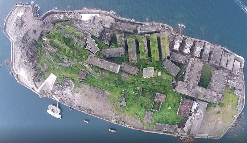
We evaluate the proposed visualization technique which can be used for building health monitoring, using measurements obtained from a sound sensor (microphone array). Figure 1 shows Gunkanjima (Hashima), a World Heritage site in Nagasaki, Japan. The microphone array is installed as shown in Figure 2 on the second floor of building No. 30 (enclosed in black circle of Figure 1(a)) of Gunkanjima. The method is applied to verify the feasibility of determining the building status by analyzing environmental sounds. Building No. 30 is the oldest reinforced concrete building in Japan and is at risk of collapsing. The microphone array is comprised of 16 microphones (each arrow in the righthand side of Figure 2 shows a cluster of four microphones).

(a)

(b)

Figure 1: (a) Bird’s eye view and (b) cityscape of Gunkanjima, Japan

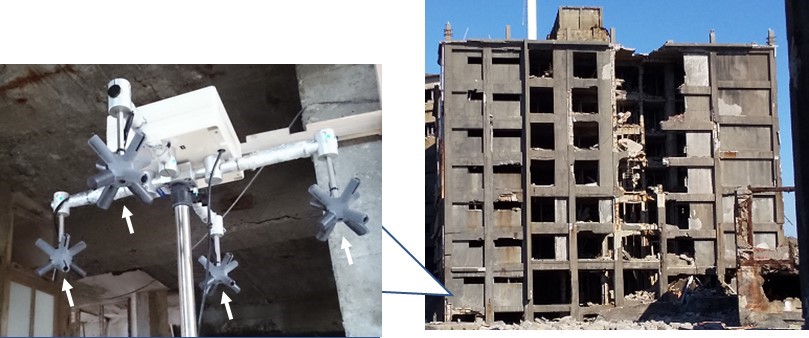Figure 2: Microphone array installed in Building No. 30 of Gunkanjima (Hashima Island), Japan.

2.2.  Sound Model of an Array with M Microphones

The sounds measured with the microphone array (Figure 2) are analyzed in the frequency domain. Then, taking the short-time Fourier transform of each microphone input at time t, the following model is obtained [3]:

y(t,w) = A(t,w)s(t,w) + n(t,w),(1)

where y(t,w) = [Y₁(t,w), …, Y_M(t,w)]^T is the input vector of the microphone array, with m-th element Y_m(t,w) of the vector, at time t and frequency w; M (= 16) denotes the number of microphones in the array; and the superscript T denotes the transpose. Additionally, A(t,w) is a matrix of transfer function vectors defined as

               A(w) = [a₁(w), …, a_L(w)],(2)

where s(t,w) = [S₁(t,w), …, S_L(t,w)]^T is the source spectrum vector of the L sound sources in the measurement environment and n(t,w) = [N₁(t,w), …, N_M(t,w)]^T, a background noise spectrum vector, carries the assumption of following a zero-mean Gaussian distribution. We assume a_i(w) = [A_1i(w),…A_Mi(w)]^T to be a transfer function that can be premeasured using time-stretched pulses [4]. We design time-stretched pulses to measure the impulse response, and the energy of the impulse signal is dispersed over time using a filter [4]. This filter is used to advance (or delay) the phase in proportion to the square of the frequency. Therefore, a_i(w) can be obtained by applying the inverse of the filter to the time-stretched pulse response.

2.3.  Sound Source Features

In building health monitoring, it is necessary to detect the location, magnitude, and duration of an eventual collapse. Hence, the loudness, continuity, and pitch features are extracted from the sounds observed by the microphone array. To visualize the sound features, a color map is drawn at the estimated sound locations to analyze the types of generated sounds. The proposed method for the building health monitoring displays information in the color map, which we call a sound map.

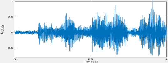Figure 3: Sample environmental sound.

The observed environmental sounds are divided into 1-second segments, as illustrated in Figure 3. The short-time Fourier transform is applied to each segment to determine the loudness, continuity, and pitch, as detailed below.

1) Loudness Feature

Loudness is important to characterize environmental sounds during building collapse. This information is represented by a sonogram, which we obtain via the MATLAB Music Analysis toolbox [5]. The estimation of the loudness per frequency band is performed using auditory models and the function ma_sone in the MATLAB toolbox, where the specific loudness sensation (in sones) per critical band (in Bark scale) is calculated in six steps. 1) The fast Fourier transform is used to calculate the power spectrum of the audio signal. 2) According to the Bark scale [6], the frequencies are bundled into 20 critical bands. 3) The spectral masking effects are calculated as in [7]. 4) The loudness is calculated in decibels relative to the threshold of hearing (decibels with respect to sound pressure level—dB-SPL). 5) From the dB-SPL values, equal loudness levels in unit phones are calculated. 6) The loudness is calculated in sones based on [8]. (Regarding detail of the six steps, see [9]). Figure 4 shows the sonogram in the Bark scale of the sound depicted in Figure 3.

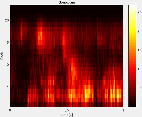Figure 4: Sonogram in Bark scale of the sound in Figure 3.

The frequency histogram of the sonogram is also computed [5], and the histogram is resampled to 8 bits using the magnitude relation for the median of the histogram. The score expressing the information can then be obtained by converting each 8-bit value into the corresponding decimal value. An environmental sound with several variations in loudness sensation per frequency band is indicated by a higher score.

2) Continuity Feature

We use pitch variations of environmental sounds with respect to time t to measure the continuity of sounds. Therefore, continuity is expressed as a score obtained from a feature representing the pitch variation of the environmental sound.

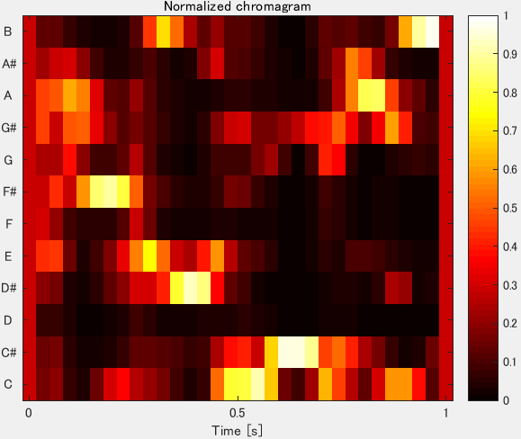Figure 5: Chromagram of the sound in Figure 3

The corresponding chromagram, like the one shown in Figure 5, can be calculated using pitch features as those illustrated in Figure 3 by applying the method in [10]. Namely, we use the MATLAB Chroma toolbox to calculate the chromagram [11]. Subsequently, a differential chromagram is determined from the initial chromagram (Figure 5) using command diff in MATLAB, and the discrete cosine transform is applied to the differential chromagram (Figure 6). Based on this result, a time-domain histogram is then calculated. Continuity information is thus represented by a score obtained from the time-domain histogram in a method analogous to that used to obtain the loudness.

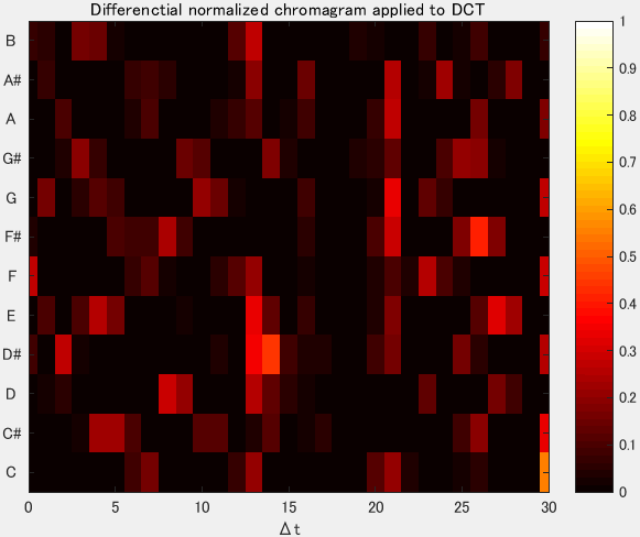Figure 6: Differential chromagram after applying discrete cosine transform for the sound in Figure 3.

The histogram represents the variation of keys over time t. Therefore, a low score suggests that key variations of the environmental sound do not occur frequently, that is, the sound has low continuity. Conversely, a high score indicates frequent key variations of the environmental sound, indicating high continuity. As environmental sounds contain various keys, we use this score to represent continuity.

3) Pitch Feature

Pitch information is represented by the corresponding score, which is used to determine the type of environmental sound.

The spectrogram of the sound depicted in Figure 3 is shown in Figure 7. Edge extraction is applied to the spectrogram allowing the calculation of the number of pixels in its frequency feature areas and centroid frequencies. The improved affinity propagation method [12] is used to categorize the detected frequency characteristic areas of the spectrogram. More details on affinity propagation can be found in [13] and [14].

Each centroid frequency obtained by improved affinity propagation is classified into low-, medium-, or high-frequency groups. Then, a frequency group histogram can be established. The pitch is obtained from the histogram as a score, for which the calculation details can be found in [15]. A low score indicates a low dominant frequency of the environmental sound, whereas a high score indicates the presence of various frequency components.

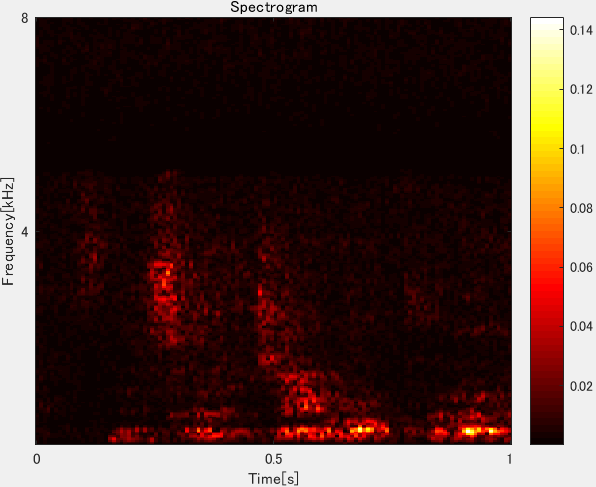Figure 7: Spectrogram of the sound in Figure 3.

2.4.  Sound Localization

Various methods for estimating sound source directions has been proposed (e.g., [16], [17], [18]) . In this paper, using A(ω) obtained from (2), the MUSIC [19] is used to estimate the locations of sound sources. Details about the estimation of virtual 3D sound source positions can be found in [10].

2.5.  Sound Map from Features

The loudness, continuity, and pitch scores are used to construct a sound map by representing the three scores in a red–green–blue color model. The obtained colors are then overlaid on the estimated sound source positions. Therefore, unlike conventional sound visualization methods such as power spectrum, the proposed sound map reflects not only the pitch but also the loudness and continuity of the sound in a color model, thus establishing a novel representation.

3.      Experimental Results

3.1.  Experimental Setup

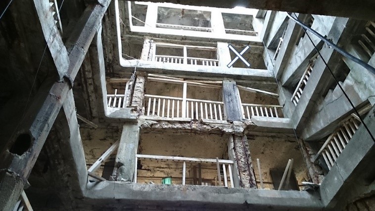
The effectiveness of the proposed method is evaluated by using the sounds of falling cans and stones measured by the microphone array installed as shown in Figure 2.

Figure 8: Experimental scenario using falling cans and stones that hit the second floor of the building as sound sources

The three hitting points for evaluation are marked with an X in Figure 8 and are located on the 2nd floor of the building. The cans are dropped from the 4th and 6th floors of the building to investigate the difference in the sound features caused by the drop height. Figure 8 also shows the placement of the microphone array and the person in charge of dropping the cans and stones.

3.2.  Sound Maps

Figure 9 shows the sound maps obtained from the sound sources generated by cans (Figure 9(a)) and stones (Figure 9(b)) hitting on the second floor. The color differences mainly correspond to loudness and continuity, as listed in Table 1, where each feature score is the average across nine trials. There is also a difference in pitch. Hence, the sounds of hitting stones have more frequency components than those of hitting cans. The three extracted features allow to distinguish differences in objects that cause sudden sounds, and Figure 9 also demonstrates the correct localization of the sound sources.

(a)

(b)

Figure 9: Sound maps of sound sources generated by (a) cans and (b) stones hitting the 2nd floor of the building. The red circle indicates the position of the microphone array.

Table 1: The averages of loudness, continuity, and pitch scores for the sounds generated by falling cans and stones hitting on second floor of the building.

	Loudness score	Continuity score	Pitch score
Can	158.2	107.3	19.2
Stone	115.3	179.8.8	32.2

(a)

(b)

Figure 10: Sound maps of the sound sources of dropping cans at the (a) 4th and (b) 6th floors of the building.

Therefore, if there are frequency differences in sounds generated before and after a building collapses, the three features, especially the pitch, can be used to detect them.

Figs. 10 shows the sound maps of the dropping cans from the fourth (Figure 10(a)) and sixth (Figure 10(b)) floors of the building, respectively, averaged across three trials. The X marks in Figure 11 show the corresponding dropping points for the maps in Figure 10. As expected, the colors on the estimated directions of the sound sources for both floors are similar.

(a)

(b)

Figure 11: Dropping points of cans (X marks) from the (a) 4th and (b) 6th floors of the building.

Table 2: Averages of loudness, continuity, and pitch scores for the generated sounds of falling cans at the 4th and 6th floors of the building.

Floor	Loudness score	Continuity score	Pitch score
2	240.0	113.7	25.0
4	240.0	84.3	16.3
6	245.3	28.3	26.0

The colors of the sound maps in Figs. 10(a) and (b) reflect the difference in floors and are mainly related to variations in the continuity score, as listed in Table 2.

The experimental results indicate the feasibility of using the proposed method for visualizing sound features in a building health monitoring system that can roughly determine the locations and types of environmental sounds in buildings.

4.      Discussion and Conclusions

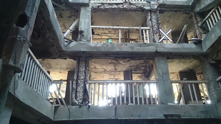
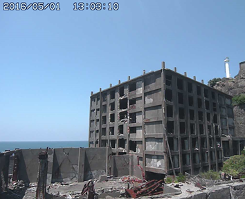
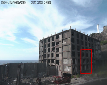
Figure 12 shows snapshots of building 30 before (Figure 12(a)) and after (Figure 12(b)) a floor collapse (red area). These snapshots illustrate the difficulty in determining the collapse through the use of images from cameras. Thus, the use of sounds may allow effective monitoring of buildings such as those in Gunkanjima, which is an uninhabited island.

(a)

(b)

Figure 12: Building No. 30 (a) before and (b) after the collapse of the floor (red area).

We propose a method of visualizing sounds which can be used for implementing building health monitoring by calculating the direction and features of environmental sounds. The proposed visualization technique of sound features considering sound localization relies on sound maps that reflect the loudness, continuity, and pitch of multiple sounds.

Experiments considering falling cans and stones were considered to simulate sounds of a collapsing building. The experimental results suggest that, using the proposed method, collapsing floors and walls attributable to the damage and deterioration of buildings can be localized. Moreover, the mechanism of building collapse may be analyzed and clarified by using the proposed method.

The proposed method for building health monitoring using the sound measurement will be used to continuously monitor building No. 30 of Gunkanjima, Japan, and the building monitoring data will be collected. In addition, we will further improve the accuracy of sound localization.

Conflict of Interest

The authors declare no conflict of interest.

Acknowledgment

This work was partly funded by Japan Society for the Promotion of Science (grant number 16H02911 and 17HT0042) and JST CREST under grant JPMJCR18A4.

1. S.A.H. Lim, J. Antony, “Statistical process control readiness in the food sector: Development of a self- assessment tool,” Trends in Food Science and Technology, 58, 133-139, 2016, doi:10.1016/j.tifs.2016.10.025.
2. M. Dora, X. Gellynck. “Lean six sigma implementations in a food processing SME: A case study,” Quality and Reliability Engineering International, 31, 1151–1159, 2015, doi:10.1002/qre.1852
3. V. R. Sreedharan, R. Raju, M. V. Sunder, J. Antony, “Assessment of lean six sigma readiness (LESIRE) for manufacturing industries using fuzzy logic,” International Journal of Quality and Reliability Management, 36(2), 137–161, 2019, doi:1108/IJQRM-09-2017-0181.
4. L. B. M. Costa, M. G. Filho, L. D. Fredendall, F. J. Gómez Paredes, “Lean, six sigma and lean six sigma in the food sector: A systematic literature review,” Trends in Food Science and Technology, 82, 122– 133, 2018, doi:10.1016/j. tifs.2018.10.002.
5. L. Marrucci, M. Marchi, T. Daddi, “Improving the carbon footprint of food and packaging waste management in a supermarket of the Italian retail sector,” Waste Management, 105, 594-603, 2020, doi:10.1016/j.wasman.2020.03.002.
6. L.B.M. Costa, M. G. Filho, L. D. Fredendall , G.M.D Ganga, “The effect of lean six sigma practices on food sector performance: Implications of the Sector’s experience and typical characteristics,” Food Control, 112, 2020, doi:10.1016/j.foodcont.2020.107110
7. J. A. Garza-reyes, I. E. Betsis, V. Kumar, M.A.R. Al-Shboul, “Lean readiness-the case of European pharmaceutical manufacturing industry,” International Journal of Productivity and Performance Management, 67(1), 20-44, 2018, doi: 10.1108/IJPpm-04-2016-0083
8. B.V. Chowdary, D. George, “Improvement of manufacturing operations at a pharmaceutical company: a lean manufacturing approach,” Journal of Manufacturing Technology Management, 23 (1), 56-75, 2012, doi: 10.1108/17410381211196285.
9. A. A. Armenakis, S. G. Harris, K. Mossholder, “Creating readiness for organizational change,” Human Relations, 46, 681–703, 1993,doi:10.1177/001872679304600601.
10. Z. Radnor, 2011. “Implementing lean in health care: making the link between the approach, readiness and sustainability,” International Journal of Industrial Engineering and Management, 2(1), 1-12, 2011, doi: 10.1016/j.socscimed.2011.01.011.
11. J. Antony, “Readiness factors for the lean six sigma journey in the higher education sector,” International Journal of Productivity and Performance Management, 63(2), 257–264, 2014, doi:10.1108/IJPPM-04-2013-0077
12. C.Andrea, and M. Kumar. “Lean Six Sigma and Industry 4.0 integration for Operational Excellence: evidence from Italian manufacturing companies.” Production Planning & Control, 32 (13), 1084-1101, 2020, doi:10.1080/09537287.2020.1784485
13. E.H. Jacobson, “The effect of changing industrial methods and automation on personnel,” Paper presented at the Symposium on Preventive and Social Psychology, Washington, DC, 1957.
14. S. Al-Balushi, P.J. Sohal, P.J. Singh, A. Al Hajri, Y.M. Al Farsi,R, Al Abri, “Readiness factors for lean implementation in healthcare settings – a literature review,” Journal of Health Organization and Management, 28(2), 135-153, 2014, doi: 10.1108/JHOM-04-2013-0083.
15. B.J. Weiner, “A theory of organizational readiness to change,” Implementation Science, 4(1), 67, 2009, doi: \10.1186/1748-5908-4-67.
16. E. Drohomeretski, S. E. G. da Costa, E. P. de Lima, P. A. Garbuio, “Lean, six sigma and lean six sigma: An analysis based on operations strategy,” International Journal of Production Research, 52(3), 804–824, 2014, doi:10.1080/00207543.2013.842015.
17. C. Robson, K. McCartan, Real world research (4th ed.), John Wiley & Sons, 2006.
18. M. B. Miles, A. M. Huberman, Qualitative data analysis: An expanded sourcebook., Sage Publications, 1994
19. M. Q. Patton, Qualitative research and evaluation methods, Thousand Oaks, Sage, 2002.
20. M. Filho, GMD. Ganga, A. Gunasekaran, “Lean manufacturing in Brazilian small and medium enterprises: Implementation and effect on performance,” International Journal of Production Research, 7543, 1–23, 2016, doi: 10.1080/00207543.2016.1201606.
21. M. Dikko, “Establishing construct validity and reliability: Pilot testing of a qualitative interview for research in takaful (islamic insurance),” The Qualitative Report, 21, (3), 521- 528, 2016, doi: 10.46743/2160-3715/2016.2243.
22. R. Bogdan, S.K. Biklen, Qualitative research for education: An introduction to theories and methods, Pearson A & B, 2007.
23. E. Guba, “Criteria for assessing the trustworthiness of naturalistic inquiries,” Educational Technology Research and Development, 29(2), 75-91, 1981, doi:.
24. M.A. Abernethy, M. Horne, A.M. Lillis, M.A. Mallina, F.H. Selto, “A multi-method approach to building causal performance maps from expert knowledge,” Management Accounting Research, 16(2), 135-155, 2005, doi: 10.1016/j.mar.2005.03.003.
25. I. Pyrko, V. Dörfler, “Using causal mapping in the analysis of semi-structured interviews,” In Academy of Management Proceedings , 2018(1), 2018, doi: 10.5465/ambpp.2018.14348abstract.
26. A. J. Scavarda, T. Bouzdine?Chameeva, S. M. Goldstein, J.M. Hays, A. V. Hill, “A methodology for constructing collective causal maps,” Decision Sciences, 37(2), 263-283, 2006, doi: 10.1111/j.1540-5915.2006.00124.x.
27. K. Jayaraman, T. Leam Kee, K. Lin Soh, “The perceptions and perspectives of lean six sigma (LSS) practitioners,” The TQM Journal, 24(5), 433–446, 2012, doi: 10.1108/17542731211261584.
28. V. F., Vallejo, J. Antony, Douglas, J. A., Alexander, P., & Sony, M. (2020). Development of a roadmap for Lean Six Sigma implementation and sustainability in a Scottish packing company. The TQM Journal.
29. J. Rockart, “Chief executives define their own data needs,” Harvard Business Review, 57(2), 1979.
30. A. Panwar, B.P. Nepal, R. Jain, A. P. S. Rathore, “On the adoption of lean manufacturing principles in process industries,” Production Planning & Control, 26(7), 564–587, 2015, doi: 10.1180/09537287.2014.936532.
31. A. Gurumurthy, P. Mazumdar, S. Muthusubramanian, “Graph theoretic approach for analyzing the readiness of an organization for adapting lean thinking: a case study,” International Journal of Organizational Analysis, 21(3), 96-427, 2013, doi:10.1108/ IJOA-04-2013-0652.
32. Y. Lagrosen, R. Chebl, M. Rios Tuesta, “Organizational learning and six sigma deployment readiness evaluation: A case study,” International Journal of Lean Six Sigma, 2(1), 23–40, 2011, doi: 10.1108/20401461111119431.
33. S.C. Cross, “Lean cuisine.” Industrial Engineer, 41(1), 46-47, 2009
34. P.B. Keliji, B.S.D Abadi, M. Abedini, “Investigating readiness in the Iranian steel industry through six sigma combined with fuzzy delphi and fuzzy DANP,” Decision Science Letters, 7, 465–480, 2018, doi: 10.5267/j.dsl.2018.1.001.
35. M. N. Mishra, “Identify critical success factors to implement integrated green and lean six sigma,” International Journal of Lean Six Sigma, 2018, doi:10.1108/IJLSS-07-2017-0076.
36. T. Y. Lee, W. K. Wong, K. W. Yeung, “Developing a readiness self-assessment model (RSM) for six sigma for China enterprises,” International Journal of Quality and Reliability Management, . 28(2),169–194, 2011, doi: 10.1108/02656711111101746.
37. A. Cox, D. Chicksand, M. Palmer, “Stairways to heaven or treadmills to oblivion?: Creating sustainable strategies in red meat supply chains,” British Food Journal, 109, 2007, doi:10.1108/00070700710780689
38. C. A. Moya, D. Galvez, L. Muller, M. Camargo, “A new framework to support lean six sigma deployment in SMEs,” International Journal of Lean Six Sigma, 10(1), 58–80, 2019, doi:10.1108/IJLSS-01-2018-0001.

(Click Here)