1. Introduction

According to [1], energy security and green economy are becoming paramount today; as a result, the demands for renewable and alternative energy sources such as solar, wind, hydro energy, bio-fuels and fuel cells, as well as energy efficient loads, are on the rise in an effort to ensure energy sustainability and carbon free environment. In this regards, we investigated thermoelectricity as a potential alternative energy for sustainable energy source and loads − that is, as a clean DC power source for low energy lighting/applications and as well to provide clean cooling/heating in various human habitats. Thermoelectricity as reviewed in [2], practically focuses on the Seebeck and Peltier effects. Seebeck effect is basically converting heat to DC electricity and the device that does this is a thermoelectric generator (TEG). The reversed phenomenon is a Peltier effect − which is basically the production of cold from DC electricity and if the direction of current flow changes (swap voltage polarity),

heat is also produced and the device that does this is called a thermoelectric cooler (TEC). Therefore, by efficiently applying thermoelectricity prudently, a clean alternative energy source for DC low power applications using TEGs and or energy efficient loads in the forms of heat pumps, air conditioners, refrigerators etc using TECs; can be passably implemented to help sustain some human habitats basic energy consumption such as lighting, cooling and heating; as well as reduce environmental pollution.

As already examined in [2], thermoelectricity lends itself to various applications with focus on how TEGs and TECs can be used respectively as a power source and as a load. Furthermore, studied in [3], is a re-configurable TEG DC-DC converter for maximum TEG energy harvesting in a battery-powered wireless sensors network (WSN). Described in [4], is the analysis and design of a thermoelectric energy harvester (TEH) prototype for powering up outdoor sensors and devices. Solar energy was harvested using different TEG arrays in [5] and a theoretical analysis of implementing a re-configurable TEG was researched in [6]. Electronic cooling was investigated in [7] and the findings revealed that the TEC cooling capacity could be increased by increasing its cold side junction temperature and decreasing its temperature difference. A multi-stage TEC module in cascade was examined in [8]; whereas in [9], an extensive mathematical analyses were articulated for TEG and TEC design and materials. A TEG model was developed in [10] for maximum power point tracking but lacks the detailed underlining maths and the parallel TEG combinations was limited to just 2. A comprehensive TEG and TEC models with the detailed maths supporting the TEG and TEC models, were presented respectively in [11] and [12].  In [13], a modeling of TEG using Modelica is asserted but deficient in the comprehensive maths, especially considering modeling infinite multiple TEGs and as well TECs modules －which were not articulated. A parametric ANSYS study of TEG and TEC was presented in [14]; however, the detailed maths and especially for the case for infinite TEG and TEC modules use/ connection, was inadequate. In addition, for large scale TEGs and TECs applications, the following studies were examined. In [15], 600 TEGs with a temperature difference of ~120 ℃, were applied to harvest and generate up to 1 kW of DC power from geothermal heat. It was further indicated a 2 kW power could be achieved with a higher temperature difference and also the TEG cost is much lower to generate equivalent amount of power than using photovoltaic. However, the study lacks the theoretical details to substantiate it. TEG harvesting of waste thermal energy from household heat sources such as a generator exhaust pipe and a kerosene stove, were performed in [16] and various parameters measurements were made but without detailing the maths to calculate these parameters. Light and heat from the Sun are the most common forms of energy abundant on Earth; as a result, [17] reviewed the possibility of integrating photovoltaic and TEG in a hybrid photovoltaic-TEG system and further examined the efficiency improvement. A 128 TEGs system was assembled in [18] to generate ~684 W of power from radiation heat transfer at a temperature difference of ~125 K and with a corresponding power density of 845 W/m2. Their results further justified that with a greater practical temperature difference of 200 K, the respective generated power and power density of their TEGs system could attain 1.23 kW and 1.51 kW/m2. Their TEGs system open circuit voltage, its output power, its power density and its conversion efficiency were investigated in details at different temperature differences; however, the underlining maths was not elaborated. A grid-tied 20 W TEG experimental model using 24 modules in series with the heat harvested from a waste incinerator, was experimented in a lab and the preliminary and analytical models of the electric output power as a function of specific temperatures, were investigated in [19]. A micro combined cold, heat and power system for a small household with a TEC as the cooler and achieving a cooling power of 26.8 W, was presented in [20]. In [21], a 3D printable TEG device architecture with a high thermocouple density of 190 per cm² by using a thin substrate as an electrical insulation between the thermoelectric elements, resulted in a high-power output of 47.8 µW/cm2 from a 30 K temperature difference. A stove-powered TEG (SPTEG) was used in [22] to generate power from waste heat released during cooking. They researched series and parallel TEGs connections and the effect of pressure to address low power output due to irregular temperature. Finally, an experimental and a numerical investigations on TECs for comparing air-to-air and air-to-water refrigeration were investigated in [23], with the findings revealing that air-to-water achieves 30-50% efficiency, compared to air-to-air cooling.

 These are just a few noted studies; however, lacking in the TEGs/TECs literature are comprehensive details on their maths, modeling and operations when connected in series and also in parallel to increase the output power (in the case of TEG) and the cooling power (in the case of TEC). This article therefore, expands on i) developing and expressing further the theoretical maths covering TEGs and TECs various parameters/modules with focus on the total internal resistance, ii) the modeling of multiple TEGs and TECs modules focusing on their electrical parameters and finally iii) their static and dynamic simulations with focus on the optimal operation points investigation as well as the interpretations thereof. The results are then validated with established published studies and concluding remarks are drawn.

2. TEGs and TECs Mathematical Analyses and Modeling

In [9], [11] and [12], the standard static mathematics defining various TEG and TEC parameters as well as their modeling are demonstrated. We developed further and present in the following sections: i) TEGs and TECs maths and ii) the implemented models (based on their maths) using Matlab/Simulink and the simulations  of TEG/TEC modules, be it in series and or in parallel connections.

 2.1 TEGs and TECs Steady-state Mathematical Analyses

The derivations thus far of the TEG and TEC parameters have been based-on the p-n junction thermoelement resistance at the thermocouple level and by extension at the module level as indicated in [9], [11] and [12]. However, in practice, more than one TEG and TEC modules will be needed for more power production and this will take the form of series and or parallel connections; as a result, the electrical resistance will often change. This section redefines the change in R to Rt and is articulated next.

TEGs Steady-state Mathematical Analysis

The following TEG parameters mathematics are developed and presented step-wise for multiple TEGs case as follows:

Thermoelectric (TE) device p-n junction thermocouple      resistance (r)

The TE device p-n thermocouple resistance r in ohm is:

r = pL/A                        (Ω)                         (1)

with ρ being the TEG/TEC electrical resistivity in Ω.m, L is the length in (m) of the TEG/TEC p-n thermocouple and the TEG/TEC p-n thermocouple area is A in metre squared (m2).

TE device (TEG and TEC) module resistance (R)

The resistance in (Ω) of a TEG/TEC module is computed as:

R = nr                    (Ω)                         (2)

where n (which differs, could be 100, 127, 199, 255 etc) is a TEG/TEC manufacturer p-n thermocouples amount used in a TEG/TEC. The more the n, the more powerful is the TEG/TEC.

 TEG/TEC module(s) total resistance (Rt)

The total resistance Rt in (Ω) of a TEG/TEC module(s) is simply calculated as:

with Tp being the TEGs/TECs (TEG/TEC modules) amount connected in parallel and Ts the TEGs/TECs (TEG/TEC modules) amount connected in series. NB: all the TEGs/TECs used in (3), have to be identical model to make sure the R of each TEG/TEC is not vastly different; if not, (3) would be inaccurate.

TEG(s) output voltage (Vo)

The TEG(s) voltage generated in volt, can be derived as:

Vo = nS∆T – IRt  (V)                         (4)

with S being the TE device Seebeck coefficient in V/K,  ∆T = Th – Tc the TEG(s) temperature difference in kelvin or °C and the output current of the TEG(s) is I in ampere.

TEG(s) output current (I)

The TEG(s) generated current I in ampere is deduced as:

with RL being the resistance of the electrical load connected to the TEG(s) output. NB: more I causes the TEG(s) more Joule heating, which negatively affects the TEGs efficiency.

TEG(s) hot-side heat absorbed (Qh)

TEG(s) produce DC power when their hot-side is at a high temperature Th, during which the TEG(s) becomes hotter and the absorbed heat in watt is Qh, given as:

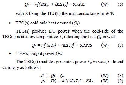
 TEG(s) electrical/conversion/thermal efficiency (ɳ)

ɳ is the TEG(s) power output Po divided by the TEG(s) hot-side heat absorbed Qh. ɳ being a performance parameter is:

TEGs maximum power conversion efficiency (ɳmp)

As a function of temperatures and Z, ɳmp is the efficiency of the TEG at its maximum output power Po − that is, at Rt = RL.

ɳmp = ɳc/[2 – 0.5ɳc+ (2/Z\bar{T}) (1+Tc/Th)]       (14)

TEG(s) maximum power output (Pomax)

The TEG(s) maximum transfer of power theoretically happens at Rt = RL. NB: in practice, Rt = RL is hardly ever the case.

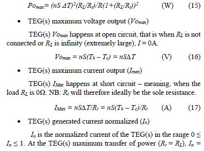
Simply, In is the TEG(s) generated current divided by the TEG(s) maximum current output. It is calculated as:

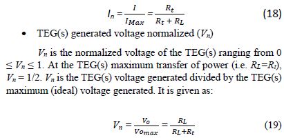
TEG(s) output power normalized (Pn)

Pn is the normalised TEG(s) power bounded between 0 ≤ Pn ≤ 1. Pn = 1 at the TEG(s) maximum transfer of power (RL=Rt). Pn is the TEG(s) power generated divided by the TEG(s) maximum output power. It is expressed as:

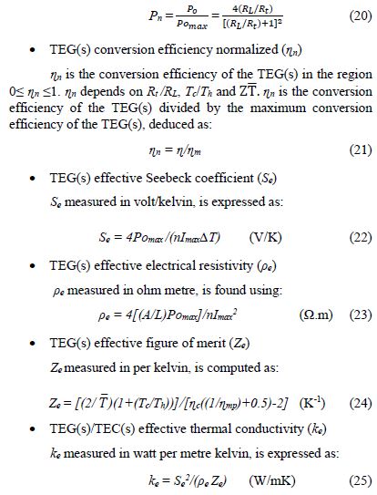
TEGs/TECs effective parameters enable researchers to factor in TEGs/TECs system losses using maximum parameters to bridge the theoretical and measured specifications differences [9].

TEG(s) Heat Flux Density (HFD)

HFD is the amount of heat absorbed per TEGs hot-side surface area (TEGsa) in watt per centimetre square.

This concludes the TEG(s) modules static mathematical analysis.

(II)    TECs Steady-State Mathematical Analysis

The following TEC parameters mathematics are examined and developed step-wise for multiple TECs case as follows:

TEC(s) voltage input (Vin)

The TEC(s) applied voltage in volt, is expressed as:

TEC(s) current to yield CoP (Icop)

                    Icop is the TECs input current in (A) needed to attain CoP.

TEC(s) maximum input voltage (Vinmax)

Vinmax is the maximum Vin in volt, that produces maximum ∆Tmax when Iin = Imax, Rt=0, Tc = 0, Qc = 0 and Th is maximum.

 

TEC(s) normalized temperature difference (∆Tn)

TECs ∆Tn, is ∆T divided by ∆Tmax and it is expressed as:

2.2 TEGs and TECs Modelling and Simulations

Covered in Section 2.1., are the TEGs and TECs parameters of interests －which were extensively expressed mathematically with emphasis/basis on the total internal resistance Rt－which was derived and the regular TEG/TEC equations re-expressed based-on Rt to now cover TEG(s)/TEC(s). The above equations are herein further modeled in Matlab and Simulink, to institute the TEGs and TECs models that can now be utilized to simulate and investigate many connected TEGs and TECs optimal performance. Exemplified in Figures 1a and 1b, are the TEGs static and dynamic simulated model GUIs, from which the TEGs parameters expressed in Section 2.1.I, can all be statically and dynamically configured for an infinite amount of TEGs connections and then simulated to obtain the TEG(s) optimum operation points. Figures 1c and 1d zoom-in on the TEGs internal modeling. Figure 1e expands on the TEGs Rt modeling − this must be matched to the load resistance RL − which can be changed before or while the simulation is running to match the TEGs Rt for maximum power transfer simulation. Figure 2 exemplifies the TECs simulator user interface. Also, multiple TECs combinations in Ts and Tp and the various parameters presented in Section 2.1.II, can be optimally simulated. Likewise, maximum power will be transferred also from the DC power supply to the TECs by matching its Rt to Rs.

Figure 1a: TEG(s) static simulator user’s interface − shows the steady-state simulation with all the input parameters fixed (though can change) over-time

Figure 1b: TEG(s) dynamic simulator user’s interface − shows the transient simulation with the Th, Tc, Ts and Tp input parameters auto changing with time

Figure 1c: TEG(s) modeling and simulation − TEG(s) parameters

Figure 1d: TEG(s) modeling and simulation − TEG(s) engine

Figure 1e: TEG(s) modeling and simulation − TEG(s) automatic internal source total electrical resistance Rt

Figure 2: TEC(s) simulator − simulates TECs various parameters by inputting a TEC specific data sheet parameters and calculates its theoretical outputs

3. TEGs and TECs Simulations Results

The TEGs and TECs simulations results are presented in three parts as follows, the i) TEGs parameters static simulation results ii) TECs parameters static simulation results and iii) TEGs parameters dynamic simulation results. Understanding these parameters operation is very paramount; otherwise, doing the physical design would just be a matter of taking chances and hoping for the best − which is sometimes the case, as most designers have reported very bad design results, likely from not understanding TE devices dynamic operations and limitations. The results from investigating the TEG(s) and TEC(s) parameters optimal operation points are discussed in details in Section 4.

3.1 TEGs Parameters Static Simulation Results

Figures 3 − 6 expound the TEGs parameters simulated to determine their optimal operation points − marked in green.

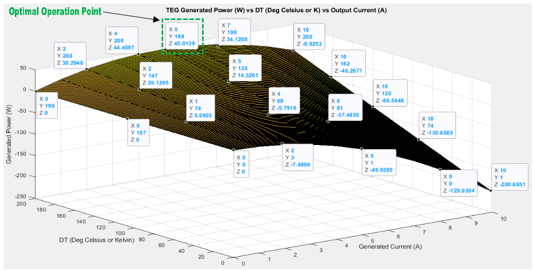Figure 3: TEG power output Po (W) vs temperature difference ∆T (°C) vs current output I (A)

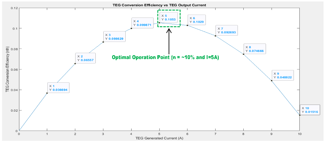Figure 4: TEG conversion efficiency ɳ vs current output I (A)

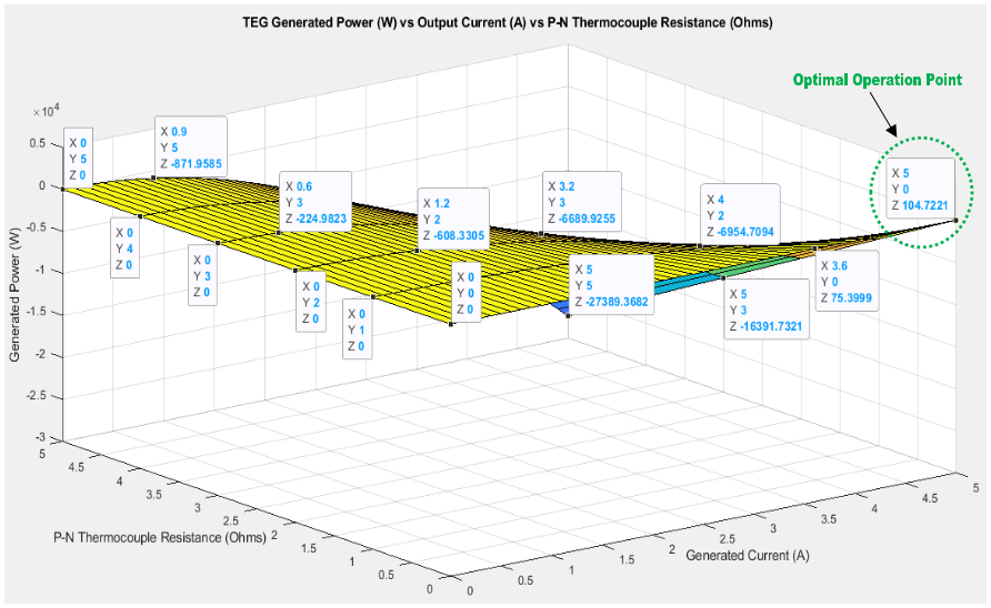Figure 5: TEG power output Po (W) vs r or R or Rt (Ω) vs current output I (A)

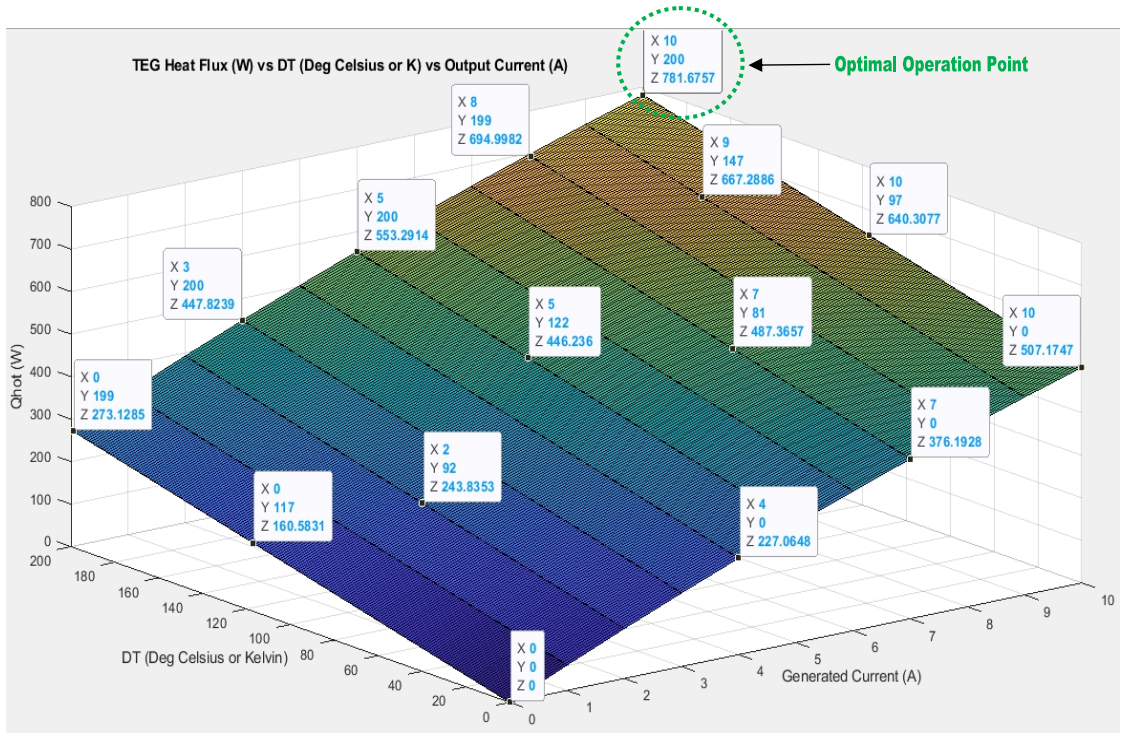Figure 6: TEG absorbed heat Qh (W) vs temperature difference ∆T (°C) vs output current I (A)

3.2 TECs Parameters Static Simulation Results

TECs parameters are simulated in Figures 7 – 10 to determine their possible optimal operation points − shown highlighted in red.

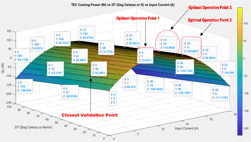Figure 7: TEC cooling power or heat absorbed Qc (W) vs temperature difference ∆T (°C) vs input current Iin (A)

Figure 8: TEC input power Pin (W) vs temperature difference ∆T (°C) vs input current Iin (A)

Figure 9: TEC input power Pin (W) vs internal resistance r or R or Rt (Ω) vs input current Iin (A)

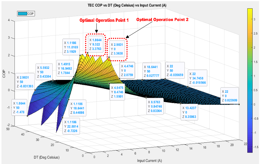Figure 10: TEC coefficient of performance CoP (%) vs temperature difference ∆T (°C) vs input current Iin (A)

3.3 TEGs Parameters Dynamic Simulation Results

TEG modules temperatures, its series and parallel connections dynamic simulation results are depicted in Figures 11a – 11f.

Figure 11a: 36 TEGs hot (Th) and cold (Tc) temperatures as well as temperature difference (DT) dynamics − temperature changes as simulation progresses

Figure 11b: TEGs in series (Ts), parallel (Tp) and total internal resistance (Rt) dynamics − 36 TEG modules simulated in 10 different auto reconfiguration

Figure 11c: 36 TEGs ideal output power, voltage and current dynamics; as TEGs temperatures and its 10 configurations change as simulation progresses

Figure 11d: 36 TEGs total internal resistance current, voltage and power losses dynamics; as the TEGs 10 configurations and temperatures auto change

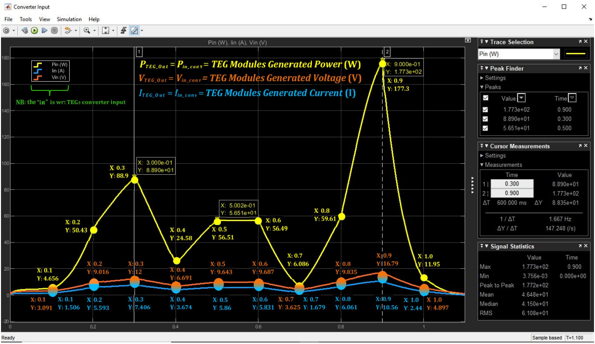Figure 11e: 36 TEGs output power, voltage and current dynamics as the TEGs temperatures and 10 configurations auto change as simulation progresses

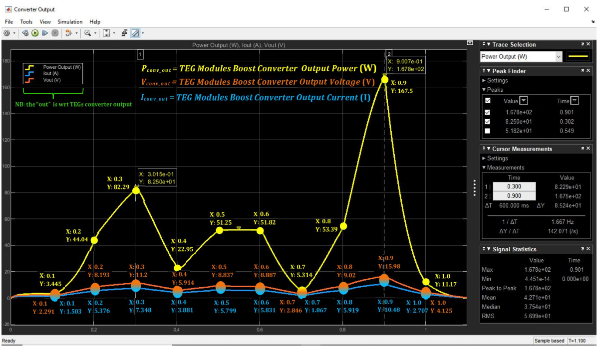Figure 11f: 36 TEGs boost converter output power, voltage and current dynamics as the TEGs temperatures and the TEGs 10 configurations auto change

4. TEGs and TECs Simulations Results Discussions

The TEGs/TECs simulations results demonstrated in Section 3, are engaged below in their following respective sub-sections.

4.1 TEGs Parameters Static Simulation Results Discussion

Some of the crucial TEGs parameters simulated in Section 3.1. and the significance of the results are herein asserted. As exemplified in Figure 3, a TEGs generated power Po is proportional to its temperature difference ∆T and output current I; however, I above 5A (in this case) will decrease Po − which is because of the TEGs internal Ohmic heating as a result of the increasing output current I. The ∆T, Po and I optimum operation points are emphasized in green in Figure 3. In Figure 4, a TEGs conversion efficiency ɳ is directly proportional to current output I up to ~5A max (in this case) and decreases later as highlighted in green. It should be noted that ɳ is as well directly proportional to Po. However, a TEG Po is reciprocally proportional to its p-n thermocouple junction resistance r and as well to its total internal resistance Rt (more than one connected TEG modules), though pro rata to I up to ~5A (in this case) as portrayed in Figure 5. At this optimal point;  Rt or R is 0Ω, I is ~5A maximum and Po is ~105W as highlighted in green. In Figure 6, the TEGs current output I is proportional directly to the TEGs absorbed heat Qh (at temperature Th on the TEG hot-side) which in turn is directly dependent on the TEG ∆T. Figure 6 pictured the optimum point stressed-out in green. It should be noted that these results are not specific to a particular TEGs’ connections − the results just fundamentally give a holistic theoretical understanding on what TEGs physical parameters must be taken into considerations, how they are interrelated, their associated dynamics and technical limitations and how they can be practically traded-off or optimized for optimal performance when designing TEGs power supply systems.

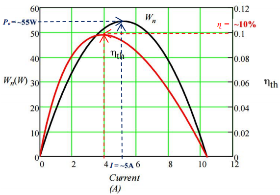Figure 12: Validating our model with [9] − TEG (i) output power PO = ~55W vs output current I = ~5A validating our Figure 3 result and (ii) conversion efficiency ɳ = ~10% vs output current I = ~ 4A  validating our Figure 4 result.

Depicted in Figure 12, is a result of a typical TEG model simulated with Mathcad using TEG standard specifications from typical manufacturers data-sheet as presented in [9]. This was used as a benchmark to validate our TEG model simulation accuracy − which is very close, besides a few discrepancies due to minor simulation settings differences. In light of this, our implemented TEG model can be used and developed further to simulate TEGs, including infinite series and parallel connections, which are central to our research and in large scale TEGs uses.

4.2 TECs Parameters Static Simulation Results Discussion

Some of the critical TECs parameters simulated in Section 3.2. and the importance of the results are herein articulated. Figure 7 illustrates that TECs Qc on TECs cold-side Tc, is reciprocally proportional to ∆T but proportional directly to Iin up to a maximum point, after which Qc starts dropping. The reasons are due to i) Joule heating (the more Iin, the more the internal heating effect) and also ii) the second law of thermodynamics − simply put, heat flows from a hotter to a colder body; in this regards, the heating caused by the increasing Iin, increases the TECs internal temperature up to a temperature greater than that surrounding the TECs hot-side Th; consequently, heat now starts to flow from the TECs hot-side to its cold-side, thus making the cooling process (heat pumping) on the TECs cold-side inefficient. In Figure 7 and highlighted in red, the Qc, ∆T and Iin; display three optimal operation points depending on the TECs design constraints/ priorities. In option 1, Qc is 115.677W with a ∆T of 1℃ and Iin of 6A. In option 2, Qc is 110.668W with a ∆T of 19℃ and Iin of 14A. In option 3, Qc is 105.664W with a ∆T of 4℃ and Iin of 16A. As evident, either ∆T and or Iin depending on the design constraints, can be optimized by either minimizing the TECs ∆T and or maximizing TECs Iin to increase Qc within max operational limits. In Figure 8, Pin and Iin are directly proportionally, which will initially increase Qc until a certain maximum limit, after which increasing Pin and Iin drop Qc − contrary to ∆T which is inversely proportional to Qc. The optimal operation point is highlighted in red. Figure 9 shows a TECs Pin vs Iin vs R. Normally R is set fixed when designed by the manufacturer but now, with Rt introduced, R can be fairly altered and if it is matched to Rs, maximum power will be transferred to the TEC(s); thereby, optimizing Pin and maximizing Qc as highlighted in red. Figure 10 demonstrates how CoP akin to Qc; increases with decreasing ∆T and initially with increasing I up to a maximum value and then starts decreasing, as current I increases as shown variously in Figure 10. Depending on the design constraints, two optimal CoP operation points are evident as highlighted in red − in optimal operation point 1, a CoP of 3.3763 is achievable by minimizing Iin to 1.8644A and maximizing ∆T to 9.322℃; whereas in optimal operation point 2, a CoP of 3.3638 is attainable by maximizing Iin to 2.9831A and minimizing ∆T to 0℃. Finally, our TECs model is reasonably validated by comparing a specific Qc of Figure 7 with that of Figure 13, as shown. The discrepancy is due to different TECs parameters setting. In sum, understanding the theory of TECs parameters and taking the various operational dynamics involved into considerations are very crucial in TEC(s) design/performance.

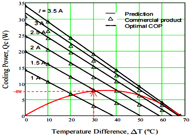Figure 13: Validating our model with Lee, 2016 [9] − using TEC cooling power Qc = ~8W vs input current I = ~1.5A vs ∆T= ~30℃ to validate our TECs Qc in Figure 7  result with cooling power Qc = ~16W vs input current I = ~2A vs ∆T= ~30℃.

4.3 TEGs Dynamic Simulation Results Discussion

Some of the critical TEGs dynamic simulated in Section 3.3. and the importance of the results are herein discussed. The TEGs temperatures and modules electrical connections (series, parallel, series/parallel) dynamics were simulated. In which beginning with the TEGs temperature dynamics, various arbitrary temperatures on the TEGs hot and cold sides as demonstrated in Figure 1b and Figure 11a, as well as summarized in Table 1, were simply dynamically simulated using time-series inputs. As expected, the TEGs dynamically generated power, voltage and current; increased with increasing Th and DT but with decreasing Tc.

Table 1: TEGS time-series inputs dynamic simulations results summary

Parameters	Matlab / Simulink Simulation Time
	0.1	0.2	0.3	0.4	0.5	0.6	0.7	0.8	0.9	1.0
Figure 11a	TEG modules Th, Tc and DT dynamic temperature inputs in ℃
TEGs Th	60	120	125	75	100	80	65	85	200	150
TEGs Tc	10	20	25	30	35	15	40	0	5	45
TEGs DT	50	100	100	45	65	65	25	85	195	105
Figure 11b	36 TEG modules in 10 dynamic Ts, Tp, Tt and Rt  auto configuration
Ts	36	18	12	9	6	6	4	3	2	1
Tp	1	2	3	4	6	6	9	12	18	36
Tt	36	36	36	36	36	36	36	36	36	36
Rt  (Ω)	54.86	13.72	6.096	3.429	1.524	1.524	0.677	0.381	0.169	0.0423
Figure 11c	36 TEG modules ideal (if TEGRtint = 0) power, voltage and current
TEGPocM  (W)	129.1	479.4	423.2	70.86	108.8	108.3	7.995	73.61	196.1	12.2
TEGVoc     (V)	85.72	85.72	57.15	19.29	18.57	18.57	4.763	12.14	18.57	5
TEGIoc     (A)	1.506	5.593	7.406	3.674	5.86	5.831	1.679	6.061	10.56	2.44
Figure 11d	36 TEG modules internal resistance power, voltage and current
TEGRtint      (Ω)	54.86	13.72	6.096	3.429	1.524	1.524	0.677	0.381	0.169	0.0423
PTEGRtint  (W)	124.5	429	334.3	46.28	52.33	51.82	1.909	14	18.88	0.2519
VTEGRtint  (V)	82.63	76.71	45.15	12.6	8.93	8.887	1.137	2.309	1.788	0.0103
ITEGRtint   (A)	1.506	5.593	7.406	3.674	5.86	5.831	1.679	6.061	10.56	2.44
Figure 11e	36 TEG modules generated (terminal) power, voltage and current
PTEG_Out   (W)	4.656	50.43	88.9	24.58	56.51	56.49	6.086	59.61	177.3	11.95
VTEG_Out   (V)	3.091	9.016	12	6.691	9.643	9.687	3.625	9.835	16.79	4.897
ITEG_Out     (A)	1.506	5.593	7.406	3.674	5.86	5.831	1.679	6.061	10.56	2.44
Figure 11f	36 TEG modules boost converter output power, voltage and current
Pconv_out   (W)	3.445	44.04	82.29	22.95	51.25	51.82	5.314	53.39	167.5	11.17
Vcomv_out  (V)	2.291	8.193	11.2	5.914	8.837	8.887	2.846	9.02	15.98	4.125
Iconv_out    (A)	1.503	5.376	7.348	3.881	5.799	5.831	1.867	5.919	10.48	2.707

 

The TEG modules quantity used and most vitally in series, parallel and mixed connection were simulated, whereby as shown in Figure 1b and Figure 11b, as well as summarized in Table 1; 36 TEGs were arbitrary chosen and then arranged in 10 different combinations to study the effects of the various arrangements and when matched to a 1.524Ω electrical load. Each arrangement gives a different Rt, consequently giving different generated powers, voltages and currents. Figure 11c depicts the TEGs ideal power, voltage and current generated − assuming the TEGs Rt or TEGRtint is trivial. Figure 11d shows the power loss, voltage drop and Ohmic current due to the presence of TEGRtint. Finally, Figures 11e and 11f, show the resultant output power, voltage and current supplied to the DC-DC boost converter and from it. As apparent, more TEG modules increased the output values; however, what is more insightful is how TEGs opt to be connected and matched to a RL − to ensure maximum power is transferred between Rt and a RL.

5. Conclusions

Sustainable energy is becoming popular to supplement the traditional grid and for private use, as well as for green economy. In view of this, we proffer thermoelectricity as an alternative energy source (TEGs) as well as an energy efficient load (TECs) for assorted applications that require low DC power, cooling and heating. However, TEG and TEC require multiple units connected in series and or in parallel to provide decent output and cooling powers respectively. Usually, the uninformed perception would be trying to utilize more TEGs and TECs with the hope to get more output and cooling powers respectively. However, our findings asserted this is not really the case, since i) TEG and TEC are not entirely linear devices, especially with increasing current, ii) TEG and TEC temperature difference ∆T and current parameters have performance dynamics which must be operated within very strict optimal operation limits to guarantee efficiency and iii) TEGs and TECs total electrical resistance Rt changes − increases when connected in series and decreases when connected in parallel. Thus, the overall power and efficiency will be affected, especially if the source and load resistances are not matched to transfer maximum power. In essence, our research major contributions include formulas developed for various TEGs/TECs parameters with focus on the TEG and TEC modules total resistance Rt variations − when more than one TEG and or TEC modules are connected in infinite series and or in parallel combinations. Further contributions include detailed TEGs and TECs theoretical simulated models using Matlab/Simulink, whereby the TEGs and TECs models were used to easily simulate and investigate some thermoelectricity profound parameters performance dynamics, Rt losses and to validate some of their operation points with industry standard models. Assorted large scale practical applications of TEGs and TECs were examined and in light of their results, our future work will include embarking on an actual lab design, testing our implemented models using them and refining ours accordingly while taking the physical dynamics into account. Thereafter, a practical pilot 1kW implementation shall be devised for a low energy combined cooling, heating and power (CCHP) system − as an alternative energy green option for private use.

Nomenclature/Symbols

A                 TEG/TEC p-n junction thermocouple area in m2

CCHP         Combined cooling, heating and power

CFD            TEC(s) cold flux density in W/m

CoP            TEC(s) coefficient of performance

CoPe          TEC(s) CoP expression

CoPmax                   TECs maximum CoP

CoPmid                    TEC(s) midpoint CoP

CoPn         TEC(s) normalized CoP TEC(s)

∆T              TEG(s) temperature difference (Th – Tc) in °C or K

∆Tmax       TEC(s) maximum temperature difference in °C

∆Tn            TEC(s) normalized temperature difference

HFD           TEG(s) heat flux density in W/m2

I                  TEGs output current in ampere through the TEG(s)

Iconv_out        TEGs booster converter output current

Icop           TEC(s) current in ampere to yield CoP

Icpmax      TEC(s) maximum cooling power current in ampere

Iin              TEC module(s) input current in ampere

Iinn             TEC(s) normalized input current is the ratio of Icop    and Imax

IMax           TEG(s) maximum output current in ampere

Imax           TEC(s) maximum input current in ampere when Qc           = 0

Imid            TEC(s) midpoint current in ampere

In                 TEG(s) normalized output current

ITEGRtint     TEG ohmic current − results to TEG Ohmic or Joule        heating

ITEG_Out        TEGs generated current (input current to the boost                   converter)

K                  TEC/TEG(s) thermal conductance in (W/K)

ke                 TEG(s)/TEC(s) effective thermal conductivity in            W/mK

L                  TEG/TEC p-n junction thermocouple length in                                   meter

n                             P-N thermocouples amount used in a TEG/TEC

ɳ                  TEG(s) thermal/electrical/conversion efficiency

ɳc                Carnot efficiency

ɳe               TEG(s) conversion efficiency expression

ɳn                TEG(s) conversion efficiency normalized

ɳm              TEG(s) maximum conversion efficiency

ɳmp            TEGs max power conversion efficiency at the TEGs           maximum Po

ρ                 TEG/TEC electrical resistivity in Ω.m

ρe               TEG(s)/TEC(s) effective electrical resistivity in Ω.m

Pconv_out       TEGs booster converter output power

Pin               TEC module(s) input power in watt

Pinmid      TEC(s) midpoint input power in watt

Po               TEG(s) output power in watt − which is  Qh − Qc

Pomax        TEG(s) maximum output power in watt

Pn                TEG(s) normalized output power

PTEGRtint    TEG generated power loss − due to TEG internal         resistance

PTEG_Out       TEGs generated power (input power to the boost                       converter)

Qc               TEC module(s) cooling power on its cold-side in (W)

Qc               TEG module(s) heat emitted on its cold-side in watt

Qh           TEC module(s) heat emitted on its hot-side in watt

Qh           TEG module(s) heat absorbed on its hot-side in watt

Qcpmax                TEC(s) Icop maximum cooling power in watt

Qcmax       TECs maximum absorbable heat in watt, when ∆T =  0°C

Qcmid       TEC(s) midpoint cooling power in watt

Qcn          TEC(s) normalized cooling power is the ratio of Qc and Qcmax

r              TE device p-n thermocouples unit resistance in ohm

R             TE device (TEG and TEC) module unit resistance in  ohm

RL            TEGs electrical load resistance in Ω connected to the  TEG(s)

Rs             Power source resistance in ohm connected to the TECs

Rt            TEG/TEC module(s) total resistance in ohms

S             TE device Seebeck coefficient in V/K

Se           TEG(s)/TEC(s) effective Seebeck coefficient in V/K

\bar{T}  TE device average temperature (Th + Tc)/2 in K or °C

Tc             Temperature on TEG/TEC cold-side in °C

Th           Temperature on TEG/TEC hot-side in °C

TE            Thermoelectric

TEC        Thermoelectric cooler

TECsa    TEC cold-side surface area

TEG         Thermoelectric generator

TEGIoc       TEG ideal generated current − assuming there is no TEGRtint

TEGPocM   TEG ideal generated power − assuming there is no TEGRtint

TEGRtint   TEG internal resistance (Rt) − responsible for the                            power loss

TEGsa      TEG hot-side surface area

TEGs Tc   TEGs cold side temperature

TEGs DT  TEGs temperature difference

TEGs Th   TEGs hot side temperature

TEGVoc     TEG ideal generated voltage − assuming there is no                      TEGRtint

TEH          Thermoelectric Energy Harvester

Tp             TEGs/TECs module quantity connected in parallel

Ts             TEGs/TECs module quantity connected in series

Tt             TEG/TEC modules total quantity connected

Vcomv_out    TEGs booster converter output voltage

Vin           TEC module(s) input voltage in volt

Vinmax   TEC’s max Vin in (V) that produces max ∆Tmax when        Iin=Imax

Vinn         TEC(s) normalized input voltage is the ratio of Vin and     Vinmax

Vo            TEG module(s) output voltage in volt

Vomax    TEG(s) maximum output voltage in volt

Vn            TEG(s) normalized output voltage

VTEG_Out    TEGs generated voltage (input voltage to the boost                   converter)

VTEGRtint  TEG generated voltage drop − due to TEG internal       resistance

WSN        Wireless Sensors Network

Z               TE device figure of merit in per K

Ze             TEG(s)/TEC(s) effective figure of merit in per K

Z\bar{T}                 TE device average dimensionless figure of merit

Acknowledgment

This work was supported in parts by the Cape Peninsula University of Technology CPGS and the University of the Western Cape HySA Systems.

Data availability

Research in progress − data available upon completion.

Conflict of Interest

Authors declare no conflict of interest.

1. M.L. van der Walt, J. van den Berg, M. Cameron, “State of Renewable Energy in South Africa”, South Africa Department of Energy, Pretoria, 2017, http://www.energy.gov.za/files/media/Pub/2017-State-of-Reewable-Energy-in-South-Africa.pdf.
2. N.P. Bayendang, M.T. Kahn, V. Balyan, “A structural review of thermoelectricity for fuel cells CCHP applications,” Hindawi Journal of Energy 2020, 1-23, 2020, https://doi.org/10.1155/2020/2760140/
3. Y.-S. Noh, J.-I. Seo, W.-J. Choi, J.-H. Kim, H.V. Phuoc, H.-S. Kim, S.-G. Lee, “17.6 A Re-configurable DC-DC Converter for Maximum TEG Energy Harvesting in a Battery-Powered Wireless Sensor Node,” 2021 IEEE International Solid-State Circuits Conference (ISSCC),San Francisco, CA, USA, 266-268, 2021, doi: 10.1109/ISSCC42613.2021.9365811.
4. D. Charris, D. Gómez, M. Pardo, “A Portable Thermoelectric Energy Harvesting Unit to Power Up Outdoor Sensors and Devices,” 2019 IEEE Sensors Applications Symposium (SAS), Sophia Antipolis, France, 1-6, 2019, doi: 10.1109/SAS.2019.8705985.
5. J. Singh, P. Kuchroo, H. Bhatia, E. Sidhu, “Floating TEG based solar energy harvesting system,” 2016 International Conference on Automatic Control and Dynamic Optimization Techniques (ICACDOT), Pune, India, 763-766, 2016, doi: 10.1109/ICACDOT.2016.7877689.
6. Q. Wan, Y. Teh, P.K.T. Mok, “Analysis of a Re-configurable TEG Array for High Efficiency Thermoelectric Energy Harvesting,” 2016 IEEE Asia Pacific Conference on Circuits and Systems (APCCAS), Jeju, Korea (South), 662-665, 2016, doi: 10.1109/APCCAS.2016.7804084.
7. R. Chein, G. Huang, “Thermoelectric cooler application in electronic cooling”, Applied Thermal Engineering, 24(14–15), 2207-2217, 2004, https://doi.org/10.1016/j.applthermaleng.2004.03.001.
8. I.R. Belovski, A.T. Aleksandrov, “Examination of the Characteristics of a Thermoelectric Cooler in Cascade,” 2019 X National Conference with International Participation (ELECTRONICA), 1-4, 2019, doi: 10.1109/ELECTRONICA.2019.8825631.
9. H. Lee, Thermoelectrics: design and materials, John Wiley & Sons, Inc., Wiley, New Jersey, USA, 2016.
10. H. Mamur, Y. Çoban, “Detailed Modeling of a Thermoelectric Generator for Maximum Power Point Tracking”, Turkish Journal of Electrical Engineering & Computer Sciences, 28, 124–139, 2020, https://doi.org/10.3906/elk-1907-166.
11. N.P. Bayendang, M.T. Kahn, V. Balyan, I. Draganov, S. Pasupathi, “A Comprehensive Thermoelectric Generator (TEG) Modelling”, AIUE Congress 2020: Energy and Human Habitat Conference, Cape Town, South Africa, 1-7, 2020; Publisher Zenodo: Geneva, Switzerland, Available online 2020, http://doi.org/10.5281/zenodo.4289574.
12. N.P. Bayendang, M.T. Kahn, V. Balyan, I. Draganov, S. Pasupathi, “A Comprehensive Thermoelectric Cooler (TEC) Modelling”, AIUE Congress 2020: International Conference on Use of Energy, Cape Town, South Africa, 1-7, 2020; Publisher SSRN: Rochester, NY, USA, Available online 2021, https://ssrn.com/abstract=3735378 or http://dx.doi.org/10.2139/ssrn.3735378.
13. F. Felgner, L. Exel, M. Nesarajah, G. Frey, “Component-oriented modeling of thermoelectric devices for energy system design,” in IEEE Transactions on Industrial Electronics, 61(3), 1301-1310, 2014, doi: 10.1109/TIE.2013.2261037.
14. C. Luo, R. Wang, W. Yu, W. Zhou, “Parametric study of a thermoelectric module used for both power generation and cooling,” Renewable Energy, 154, 542-552, 2020, https://doi.org/10.1016/j.renene.2020.03.045.
15. C. Liu, P. Chen, K. Li. “A 1kW Thermoelectric Generator for Low-temperature Geothermal Resources,” PROCEEDINGS, 39th Workshop on Geothermal Reservoir Engineering, Stanford University, Stanford, California, USA, 24-26, 2014, SGP-TR-202. https://pangea.stanford.edu/ERE/pdf/IGAstandard/SGW/2014/Li.pdf [Date accessed: August 3, 2021].
16. S.O. Giwa, C.N. Nwaokocha, A.T. Layeni, O.O. Olaluwoye, “Energy harvesting from household heat sources using a thermoelectric generator module,” Nigerian Journal of Technological Development, 16(3), 2019, http://dx.doi.org/10.4314/njtd.v16i3.6.
17. M.W. Aljibory, H.T. Hashim, W.N. Abbas, “A Review of Solar Energy Harvesting Utilizing a Photovoltaic–Thermoelectric Integrated Hybrid System,” IOP Conference Series: Materials Science and Engineering, 4th International Conference on Engineering Sciences (ICES 2020), 1067, 2021, Kerbala, Iraq, doi:10.1088/1757-899X/1067/1/012115.
18. X. Hu, C. Jiang, X. Fan, B. Feng, P. Liu, Y. Zhang, R. Li, Z. He, G. Li, Y. Li, “Investigation on waste heat recovery of a nearly kilowatt class thermoelectric generation system mainly based on radiation heat transfer,” Energy Sources, Part A: Recovery, Utilization, and Environmental Effects, 2020, https://doi.org/10.1080/15567036.2020.1829190.
19. M.Y. Fauzan, S.M. Muyeen, S. Islam, “Experimental modelling of grid-tied thermoelectric generator from incinerator waste heat,” International Journal of Smart Grid and Clean Energy, 2020, doi: 10.12720/sgce.9.2.304-313.
20. M. Ebrahimi, E. Derakhshan, “Design and evaluation of a micro combined cooling heating and power system based on polymer exchange membrane fuel cell and thermoelectric cooler”, Energy Conversion and Management, 171, 507-517, 2018, https://doi.org/10.1016/j.enconman.2018.06.007.
21. A.G. Rösch, A. Gall, S. Aslan, M. Hecht, L. Franke, M.M. Mallick, L. Penth, D. Bahro, D. Friderich, U. Lemmer, “Fully printed origami thermoelectric generators for energy-harvesting,” NPJ Flex Electrons, 5(1), 2021, https://doi.org/10.1038/s41528-020-00098-1.
22. V.B. Abhijith, K. Narayanaswamy, C.M. Pooja, S.V. Prasad, R. Sambhu, “Household Application of Thermoelectric Generator in the Field of Propagating Power from Waste Heat,” AIP Conference Proceedings 2297, 020010, 2020, https://doi.org/10.1063/5.0031699.
23. F. Afshari, “Experimental and numerical investigation on thermoelectric coolers for comparing air-to-water to air-to-air refrigerators,” Journal of Thermal Analysis and Calorimetry, 144, 855–868, 2021, https://doi.org/10.1007/s10973-020-09500-6.

(Click Here)