1. Introduction

Nowadays, the energy demand is permanently increasing, causing an energy crisis due to the depletion of fossil energy sources such as coal, oil and natural gas. Therefore, the price of electricity from centralized generation keeps increasing as well. In addition, the environmental deterioration of the planet due to Greenhouse Gases emission, as well as the technological development of energy control, have made the integration of renewable energy sources more attractive for professionals as well as for individuals. These clean and abundantly available renewable power sources such as solar and wind powers, which fall under the scope of Decentralized-Generation, are currently more profitable and widely exploited, and can be used either in Grid-connected or autonomous modes. The application of PV systems has become more common in developed and growing countries, and their performances are better in high solar irradiation areas, and can provide enough power if properly operated. Due to the intermittency of climatic conditions, the output power of the Photovoltaic Generators (PVGs) is affected. This latter have enormous energy potential, even if their efficiency is relatively low (25% to 30%). Under these variable conditions, the power delivered changes according to the voltage imposed on their terminals. In order to take advantage of the fully PVGs potential, the Maximum Power Point (MPP) of the Voltage-Power curve must be reached for any solar irradiation and temperature value. Maximum Power Point Tracking (MPPT) algorithms have been developed to achieve this purpose. Several works have been carried out for MPPT algorithms development, among which stand out [1]-[4], and which differ according to a compromise between complexity and desired performances. An MPPT using Adaptive Fuzzy Logic control for Grid-connected Photovoltaic systems is presented in [5]. These MPPT algorithms are divided into two families: on the one hand those based on power derivation method such as INcremental Conductance (INC). On the other hand those based on voltage/current feedback such as the Perturb and Observe (P&O) [6]. A comparison of the dynamic and the speed of different MPPT algorithms is presented in [7]. The most commonly used MPPT algorithm is P&O due to its simple implementation and good performances [8], [9].

 One of the major advantages of PVGs is their smooth integration via existing power converters. Unfortunately, their output power is highly dependent on weather and climatic conditions. Therefore, perfect services to UG and loads, requiring constant power profiles, cannot be guaranteed. Consequently, PVG alone will not lead to satisfying results. Hence, it is either Grid-connected or associated with a storage system (Hybridation), or even with both simultaneously, to ensure supplying continuity. The storage device can be a battery-bank, fuel-cell/electrolyzer system, flywheel, super-capacitor, compressed air… and the way the energy is stored depends on the application.  As said before, solar systems can be either autonomous, or connected to the Utility Grid (UG) which represents the purpose of this paper. Grid-connected solar systems can operate either for total, or surplus sale in case of self-consumption. In both cases, a certain power will be destined to injection into the UG. Total sale system is beneficial for individuals in countries where the selling price of solar energy is higher than UG supply energy price. Other countries grant self-consumption bonuses, thus it is more beneficial to maximize the consumption of the produced solar energy, and to sell the surplus to the UG after that. Technically, the difference between these two systems lies on the metering solution. Figure 1 shows two metering solutions that can be adopted for total sale and for surplus sale. In case of total sale as shown in Figure 1(a), a no-consumption meter can be added between the DC/AC converter and the Common Couplin Point (CCP), to avoid charging the battery with the low price energy of the UG, before reselling it to the latter with higher injection price. Regarding self-consumption case, UG provides power when PVG generation is either zero or unable to satisfy the load demand. However, monthly energy bill of UG subscriber increases with the increase of its subscription power. As a result, peak shaving would be an advantageous application of the storage system for the UG subscriber. In fact, the kWh in many countries is more expensive in peak hours where energy demand is high. Peak shaving will reduce the power requested from the UG in this time period, leading to a reducing of the subscription power and the energy bill as well. It will be also beneficial in the perspective of eliminating penalties due to subscription power exceeding. Peak shaving would be beneficial also for the UG and for environment. At the UG level, the decrease in power demand reduces the risks of grid congestion, reducing as well the necessity of calling the backup centralized stations. For example, in Morocco, the kWh produced is still very polluting, given that 61% of electricity is produced from coal centralized stations [10]. Thus, at the environmental level, less demand from these stations means less Greenhouse-Gases emissions. An operating power and discharge time based comparison of different storage devices is presented in [11], and batteries are most suited for peak shaving applications. However, this storage system requires accurate regulation of charge/discharge currents within manufacturer specified range in order to increase its lifetime. Adding constraints of State Of Charge (SOC), which must be kept in a recommended range, to avoid creating harmful irreversible reactions in the battery electrodes, and hence decreasing its lifespan. Sizing properly the battery-bank is essential, in the aim of getting operational for peak shaving, as soon as the UG power requested reaches its maximum allowed power known as the subscription power. Peak shaving via batteries in France had been studied in [12], and inspired the battery-bank sizing method presented in this paper.  Figure 2 shows some metering cases that can occur for Grid-connected solar system in self-consumption mode and which are adopted in Morocco, and will constitute the basis of the development of the proposed Energy Management Strategies (EMSs) in this paper. Whatever the meter is, if solar production is either zero or insufficient to meet load demand, the metering index increases to give the electrical energy consumed in kWh to the distributor, since the deficit is provided by the UG. When the output power of the PVG exceeds the one requested, the metering index works according to the metering type:

• Digital Metering (DM) Figure 2(a): by injecting into the UG, the consumption metering index start increasing as if the individual has consumed the injected energy (concerns around 1 million Moroccan UG subscribers) [13].
• Irreversible Electromechanical Metering (IEM) Figure 2(b): by injecting into the UG, the metering index does not change because the rotation of the disc in the opposite direction is prohibited. Energy is injected and consumed in the neighborhood for free.
• Reversible Electromechanical Metering (REM) Figure 2(c): during injection, the meter index will subtract the injected energy because the rotation of the disc in the opposite direction is allowed.

It is clear that the last metering system is the most favorable for the UG subscriber. In this paper, battery integration with the aim to realize peak shaving, throughout the different metering cases presented in Figure 2, will be studied, by managing the power flows within the Grid Connected Hybrid Renewable Energy System (GCHRES). This paper deals with a Grid-connected solar system corresponding to a self-consumption operation, and as part of fair net-metering; 1kWh given for one 1kWh delivered [13], without taking into account solar energy selling and UG energy buying prices. Hence, three EMSs are proposed, depending on the metering type and on the grid injection limitation modes. Their main objective is to permanently satisfy the house loads demand. The battery charge and discharge will be carried out while respecting its technical constraints, related to its SOC and its maximum charging/discharging powers. It is noticed that the system studied do not contain dump load. The first EMS (EMS 1) targets a system equipped with either reversible or irreversible electromechanical meter, when injection into the UG is allowed without limitation. Therefore, the PVG is operating globally under the control of the MPPT algorithm. The second EMS (EMS 2) targets a system with same metering types, but in grid injection limitation case. The output power of the PVG is limited in certain cases by the mean of a limitation power point tracking algorithm, called LPPT and presented in [14]. Different LPPT control schemes are presented in [15]. The two EMS presented above are combined in one flowchart. The third EMS (EMS 3) is destined to digital metering where the subscriber will suffer financial losses in the event of an injection into the UG. Injection should be avoided at all cost. The output power of the PVG is limited in certain cases by the mean of the LPPT control. The three EMSs are presented in detail in a following section. Performances of the proposed GCHRES under the supervision of the different EMSs are simulated in MATLAB/SIMULINK using real weather data corresponding to the region of Marrakech in Morocco. This paper is structured as follow: section II presents a description of the proposed GCHRES and the control of its different components. Section III presents the battery-bank sizing method and the proposed EMSs with their different operating modes. Section IV presents and discusses the results obtained by simulation on MATLAB/SIMULINK. Finally, section V summarizes the results obtained in a conclusion.

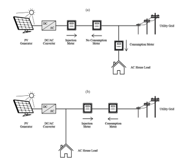Figure 1: Metering solution for Grid-Connected solar systems (a) total sale (b) surplus sale

2. System Modelling and Control

The proposed system constituting the GCHRES is illustrated in Figure 3. Its architecture based on two buses (DC and AC buses), includes a PVG, considered as the main power source intended to meet the variable demand of a house located in Marrakech, Morocco. The UG is the main backup source in the event of a PVG power deficit. A battery-bank is used for peak shaving application. The PVG and the battery, via their respective power converters, are connected to the DC-Bus. As the DC-Bus voltage is higher than the PVG voltage variation range, the interfacing between these two elements is realized via a DC-DC Boost converter. This solution makes it possible to reduce the number of solar panels constituting the PVG and thus to reduce the initial investment cost. The battery-bank voltage can be kept lower than the DC-Bus Voltage, by realizing the charge and discharge operations through a bidirectional DC/DC Buck-Boost converter (BBDC). The converter operates in Buck mode during the charge, and in Boost mode during the discharge, thus making it possible to limit the number of batteries constituting the battery-bank. The DC-Bus output is connected to the CCP combining the UG and the AC-house via an IGBT based three-phase reversible inverter called Alternative Side Converter (ASC) in this paper. A state based supervisory controls the power flows within the GCHRES.It is important to notice that in this paper, expressions including powers related to the battery, UG, PVG and the Load are presented in a way that respects the powers convention sign in MATLAB/SIMULINK. It means that all powers related to the battery charging process are positives and all the ones related to its discharging are negatives. Concerning the UG, all powers related to injection are positives and all the ones related to its consumption are negatives. Unidirectional load and PVG powers are always positives. The detailed description of each part of it, as well as the proposed EMSs will be explained in futures sections

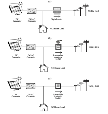Figure 2: Metering cases for Grid-Connected solar systems in Morocco (a) DM (b) IEM (c) REM

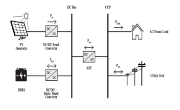Figure 3: Architecture of the proposed GCHRES

2.1.  Photovoltaic Generator Mathematical Modelling

  A photovoltaic array is the association of several photovoltaic cells. Many mathematical models of photovoltaic cell have been developed to represent their highly nonlinear behavior, caused by semiconductor junctions constituting the basis of their construction. The single diode representation presented in Figure 4 is adopted in this paper, considered as the most commonly used model [16]. The PV cell output current is given by (1). where: Photo-Current depend on solar radiation and cell temperature [A];  Diode Current ;  Shunt Resistance current .

The photo-current    is given by (2).

Where:  Short-Circuit current of the cell under STC [A];  Temperature coefficient of the short-circuit current [A /K];  Temperature of the cell [K];  Reference Temperature of the cell [K];  Solar Irradiation [W/m²];  Reference Solar Irradiation [W/m²].

The current  passing through the diode is given by (3), where [A] represents the Diode Reverse Saturation Current given by (4), and [A] given by (5) represents the Diode Reverse Saturation Current under STC.

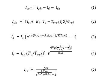where:  Diode Reverse Saturation Current [A]; q Electron Charge (1.602 x );  Cell Voltage [V];  Cell Serie Resistance [Ω];  Cell Output Current [A];  K Boltzmann Constant (1.38 x ; A Cell ideality factor dependent on PV technology; Gap energy of the semiconductor used in the cell (1.1eV for Silicon) [eV];  Cell Open Circuit Voltage [V];  Ns Number of cells connected in series.In this model,  models Joule effect Losses, while represents the losses due to the imperfect nature of materials used for solar cells making.

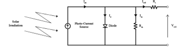Figure 4: Single diode representation of a PV cell

Several PV cells are connected to obtain a PV array. Connecting them in parallel results in a higher output current, while output voltage increases if they are connected in series. The same thing occurs when passing from PV array to PV fields constituting a PVG. Therefore, depending on the application and the load to be supplied, the PVG should consist of   array in series constituting strings and  strings connected in parallel. In this study, it is considered an  8  PVG peak power. The solar array used in the simulation is a 1SOLTECH-1STH-215P from the SIMPOWERSYSTEMS library present in SIMSCAPE in MATLAB/SIMULINK, with a peak power of  213.1  in Standard Test Conditions (STC). It corresponds to a single diode model presented above, whose input parameters are the solar irradiation and the cell temperature. The number of arrays N necessary in order to reach an overall power of about 8  is equal to 38 according to (6). By choosing and  equal to 19 and 2 respectively, the operation range of the PVG voltage will be comprises between =0V and =689V, and a DC/DC Boost converter is needed to allow the connection between the PVG output and the DC-bus of 1000V. The 8  PVG Voltage-Current and Voltage-Power curves, in STC, are presented in Figure 5(a) and Figure 5(b) respectively, depicting the PVG main characteristics.

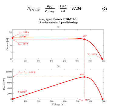Figure 5: PVG characteristics curves in STC (a) Current-Power (b) Voltage-Power

Equations (7) and (8) show the DC/DC Boost converter input/output voltages and input/output currents relations respectively. where:  DC-bus voltage [V];  PVG output Voltage [V];  Boost converter output current [A];  PVG output current [A]; D Duty Cycle of the converter.By neglecting losses, the relation between the input and output powers of the converter is given by (9). Equations (10) and (11) show the maximum and nominal powers of the DC/DC Boost converter respectively [12]. According to (7), the duty cycle increase causes the PVG voltage decrease, and its decrease results on the PVG voltage increase.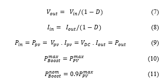

2.2.  Photovoltaic Generator Control

Depending on the EMS in operation and on the application, the PVG will have to be controlled by two different algorithms. If the fully potential of the PVG is requested, then it will be controlled by the mean of the MPPT, otherwise, if its output power must be limited, the LPPT will take over. In both cases, reaching the operating point is often achieved by introducing a DC-DC Boost Converter, which constitutes a voltage adaptation stage between the PVG output and the DC-Bus. In both cases, the control algorithm generates at its output the duty cycle of the converter, to reach the desired voltage on the PVG voltage-power curve. PWM generates the IGBT switching signals according to this duty cycle. The decision of limiting the power is given by the supervisory system according to the EMS in operation. It is possible to integrate the PVG control via the ASC, but it is not possible in this case as the PVG voltage, varying between =0V and =689V, is lower than the 1000V’s DC-Bus. The overall PVG architecture control is shown in Figure 6. The characteristics of the DC/DC Boost converter used in the simulation are summarized in Table 1.

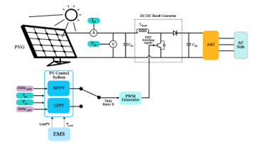Figure 6: Overall PVG control architecture

By using a P&O control algorithm, the optimal point ( , ) is reached for any value of temperature and solar radiation. The P&O algorithm corresponds to the right part of Figure 9 and its operation on the voltage-power curve is depicted in Figure 7. In case of power limitation, the PVG reference power is calculated by the supervisory system according to the EMS in operation. This power is achieved using the LPPT algorithm. As with the MPPT, the LPPT makes it possible to reach the limited power point (LPP) on the voltage-power curve, by imposing the corresponding voltage on the PVG terminals. Seen the bell shape of this curve, this power corresponds to two voltages. It is preferable to impose the greatest voltage (located on the right side of the MPP) to decrease the PVG output current, in order to decrease the Joule effect losses according to (9). The LPPT step  is reduced when entering the convergence zone (12), in order to reduce the amplitude of the oscillations around the power reference , and thus to increase tracking precision of this reference. The LPPT algorithm corresponds to the left part of Figure 9 and its operation on the voltage-power curve is depicted in Figure 8.

Table 1: DC/DC Boost converter characteristics

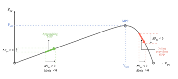Figure 7: P&O algorithm principle

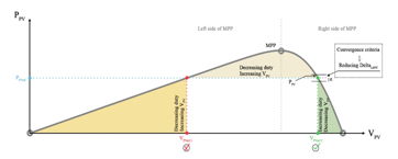Figure 8: LPPT algorithm principle

2.3.  Battery System Mathematical Modelling

      Batteries are no longer simple components with reduced number of developed models, so it is not easy to model the electrochemical interactions of a battery by simple circuits. In the literature, many models are available [17]-[20], to meet fine and

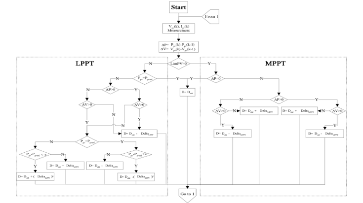Figure 9: Overall PVG control algorithm

rapid simulation needs. New dynamic models of Lead-Acid batteries are presented in [21], and take into account the dynamic character of the elements of the equivalent circuit, namely the resistance and the capacity of the main branch. In our case, a simple model is sufficient, responding properly to charge and discharge battery requests. In this study’s simulation a Lead-Acid battery is used. It is included in the SIMPOWERSYSTEM Toolbox of MATLAB/SIMULINK. The battery is modeled as a variable voltage source connected in series with an internal resistance, so the voltage across the battery is given by (13).  The internal resistance  of the battery is assumed to be constant during charge and discharge and does not change with the magnitude of the current. Contrary to this, the open circuit voltage  is different during charging and dischaching processes. It depends on the battery current  , on the capacity extracted and on the Hysteresis phenomenon of the battery. Therefore,  is given during discharging and charging processes by (14) and (15) respectively, and the instantaneous value of the SOC is given by (16), according to [22].

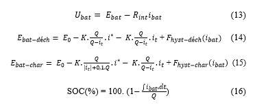where:  Voltage at the battery terminals ;  battery Open-Circuit Voltage ; battery Internal Resistance ; battery Current [A]; Constant Voltage [V]; K Polarization constant or polarization resistance; Dynamic Low Frequency current [A];  Capacity Extracted [A]; Q Maximum battery Capacity [C]; & battery current Functions representing HYSTERESIS phenomenon of the battery during charge and discharge respectively.

Equations (17) and (18) shows respectively the maximum and nominal powers of the DC/DC Boost converter [12].

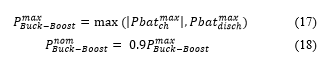where  and  are the battery maximum charging and discharging powers respectively (battery charging power is counted negatively in MATLAB/SIMULINK). Figure 10 shows the equivalent circuit of the battery according to the model described below. The characteristics of the battery-bank overall system, used in simulation are presented in Table 2, where the complementary informations concerning the battery sizing are presented in section III.

Table 2: Simulation overall battery-bank system characteristics

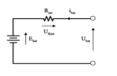Figure 10: Battery equivalent circuit representation

2.4.  Battery Bank Control

     The battery-bank is connected to the DC-Bus via a BBDC. The reference power to be delivered or received by the battery-bank is generated by the supervisory according to the EMS in operation. Then, this power is divided by the battery-bank voltage to obtain the current reference . A PI based current loop control is used to adjust the current of the battery-bank at its reference . A PWM generator generates the opposite switching signals  and  of the BBDC, according to the duty cycle D constituting the PI controller output. Figure 11 illustrates this control process.

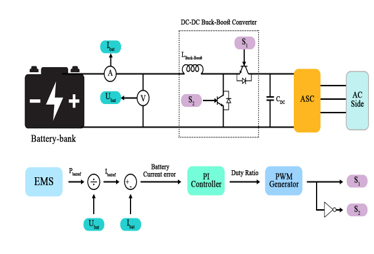Figure 11: Overall Battery-Bank control architecture

2.5.  AC Side Equations

Fig. 12 indicates the alternative side of the GCHRES. Voltage and current equations are given by (19) and (20) respectively.

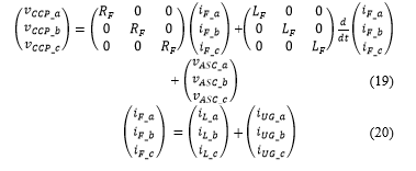where: j = (a, b, c);  currents through the ASC output filter [A];  load currents [A];  UG currents [A]; CCP simple voltages [V]; ASC output voltages [V]; respectively ASC output Filter résistance  and inductance [H].

After passing through PARK transformation, the system (19) becomes (21).

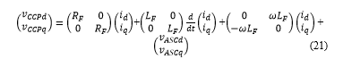where:    direct and quadrature CCP voltage components respectively [V];  direct and quadrature ASC output voltage components respectively [V];              direct and quadrature filter current components respectively [A]; UG Pulsation [rad/s].

2.6.  VOC Control of Alternative Side Converter

    Controlling the ASC aims to reach two main objectives. The first is to ensure a unity power factor on the AC-side. It means zero reactive power exchange between the ASC and the CCP. The second is to regulate the DC-Bus voltage at its reference value. Keeping its voltage constant is very important since all the power converters are connected to it. The reactive power and DC-Bus voltage references are fixed to 0VAR and 1000V respectively. DC-side current equations are given by (22), (23) and (24).

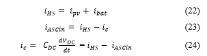where:  DC-Bus Current [A];  ASC Input Current ; Renewable Hybrid System current ; PVG Output Current ; Battery charging/discharging current [A]; DC-Bus voltage [V].

Power equations are given by (25) and (26).

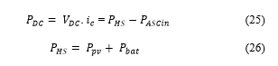
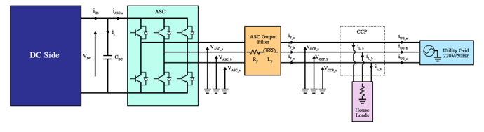Figure 12: AC-side of the GCHRES

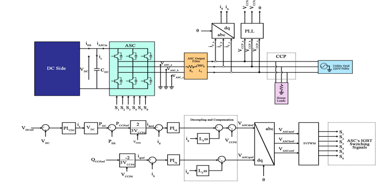Figure 13: Overall ASC control architecture

where:  DC-Bus power [W]; ASC input power ; renewable hybrid system power  ; PVG output power ; Battery charging/discharging power [W].

From (25), the DC-Bus voltage can be regulated by controlling the ASC input power . By neglecting the ASC losses, we can assume that:

VOC consists on aligning the d-axis of the (d,q) rotational coordinate system with the direct component  of the CCP voltage, thus the CCP voltages will be:

 The CCP active power is given by (30) and will be simplified to (31) according to (28) and (29).

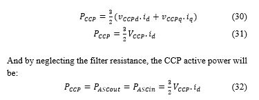
 According to (32), the ASC input power can be controlled by only controlling the d-axis current , since after aligning  with the d-axis, this latter became constant. Consequently, the DC-Bus power will be controlled too according to (25). The CCP reactive power is expressed by (33) and will also be simplified to (34) according to (28) and (29).

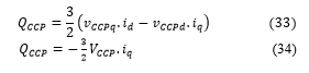Therefore, the reactive power exchange between the ASC and the CCP can be controlled by only controlling the q-axis current . According to (28) and (29) the equations system (21) becomes (35), and after passing through Laplace transformation, the system equation obtained in (36) will be used for the ASC control process

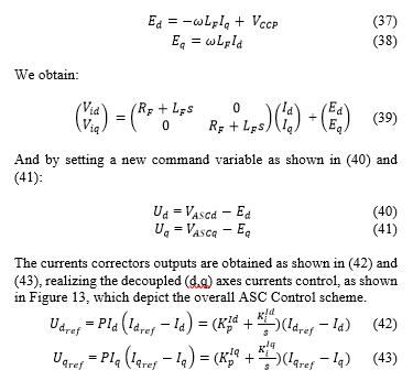
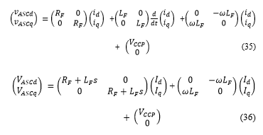According to (36), both voltages   and  act on the two currents  and . In this case the decoupled control technique will be used. By setting a new variable as shown in (37) and (38):

A PLL block is used to synchronize the ASC with the UG. Their connection requires to continuously determine the phase angle, on which the control of active and reactive powers mainly depend. PLL is an effective method for determining this angle

The principle is to use a PI corrector to regulate the q-axis CCP voltage component to a reference value equal to zero. The output of the PI block is the angular speed of the (d,q) rotational frame reference, and the angle θ is obtained by integrating this speed as shown in Figure 14. SVPWM control of the ASC is used to reduce current ripples and also the switching frequency of the converter. Equations (44) and (45) shows the maximum and nominal powers of the ASC respectively [12]. Parameters of the AC-side used in simulation are shown in Table 3.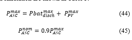

3. Battery Bank Sizing & Energy Management Strategies

3.1.  Battery Bank Sizing

      Monthly real average solar irradiation and temperature data of the region of Marrakech collected from [23] on hourly basis have been required and used for sizing the battery-bank. These data areshown in Appendix A. The average demand profile estimation for each month, on hourly basis, have been also required. As mentioned above, the battery operates for peak shaving application. Thus, it is sized according to the following criterias: maximum discharging power, maximum charging power, daily energy to be supplied and daily energy to be absorbed. The maximum power that the battery must be able to absorb/deliver are calculated via equations (46) and (47) respectively.  The minus sign in these equations are introduced to respect the battery charging and discharging powers signs convention adopted by MATLAB/SIMULINK, where ‘t’ varies on hourly basis while ‘j’ varies on monthly basis. A more proper sizing would be realized by reducing the basis of the variation of ‘t’ and ‘j’, for exemple taking a 10min basis for ‘t’ and daily basis for ‘j’ (j=1 to 365). According to Table B.1 in Appendix B, the battery maximum charging power  is around -4.9kW, which corresponds to the most favorable situation throughout the year in terms of difference between PVG generation and load demand. The battery maximum discharging power  is equal to 4.6kW, which corresponds to the worst situation throughout the year according to the same criteria. The maximum daily energy that the battery must be able to absorb and supply are given by (48) and (49) respectively. Sigma (  is a coefficient introduced to take into account only moments of the day where the battery must absorbs energy, in the maximum daily energy calculation. Unlike  lambda (  allows to take into account only the moments of the day where the battery-bank must supply energy, in the minimum daily energy calculation. These coefficients are determined by (50) and (51).

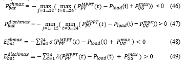
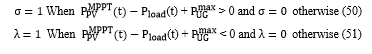Table 3: Simulation AC-side characteristics

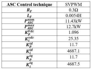
Table B.2 in Appendix B, gives the maximum daily energy that the battery must be able to absorb and supply, corresponding to an absorbing energy of -29.983kWh for the yearly most favorable case, and providing energy of 29.649kWh for the yearly worst case. Finally, the Battery bank capacity is given by equation (52).

To take advantage of the battery-bank performances without reducing its lifespan, the adopted values of    and   are ​​20% and 80% respectively, which correspond to the most often recommended values ​​found in the literature of Lead-Acid batteries. Considering a maximum depth of discharge of  = , and an operating voltage of 504V, the battery-bank capacity is given by (53).

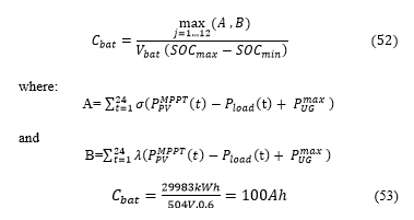Hence, 100Ah, 12V battery rating is considered and therefore 42 Batteries are required to connect in series to constitute the battery-bank.

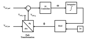Figure 14: PLL control diagram

3.2.  Energy Management Strategies

      The different operating modes of the GCHRES and its power flow management are governed by a supervisory controller through EMSs. Three EMSs are proposed in this paper and differ depending on the type of metering with the UG. As mentioned at the introduction, EMS1 is destined for systems with either reversible or irreversible electromechanical metering in the no grid limitation case. EMS2 is destined for the same metering types as EMS 1 but targets the grid limitation case. EMS 3 is destined for digital metering. The main common purpose of all these EMSs is to ensure continuity and reliability of supply to the AC-house, taking into account the battery technical constraints. Hence, they all aim to keep the SOC between a minimum and maximum values  and  respectively. The proper use of the battery avoid reducing its lifespan, avoiding as well the need of replacement of this device. All EMSs aim to charge the battery as soon as possible through the available source; PVG or UG, or both at the same time, to get always operational when requested for peak shaving. The PVG operates by default in MPPT mode, when power limitation is not required. Figure 15 depict the supervisory controller scheme. On the one hand, inputs are related firstly to the type of metering determined by METERTYPE, followed by the UG constraints in term of subscription power , and maximum injectable power in case of injection limitation (Gridlim=1). On the other hand battery constraints concern the SOC and the maximum charging/discharging powers  and  respectively.  Power measurement Inputs are the load demand power , and the net power   equal to the difference between PVG and load demand . Outputs in terms of battery power reference , and PVG power reference   in case of power limitation (LimPV=1), are generated by the supervisory controller according to the above mentioned Inputs. As mentioned before, EMS 1 and EMS 2 are combined in one flowchart presented in Figure 16, while Figure 17 is representing EMS 3.

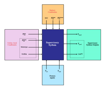Figure 15: GCHRES supervisory controller scheme

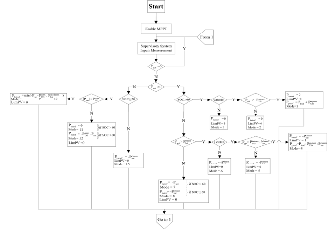Figure 16: Combined EMS 1 & EMS 2 flowchart

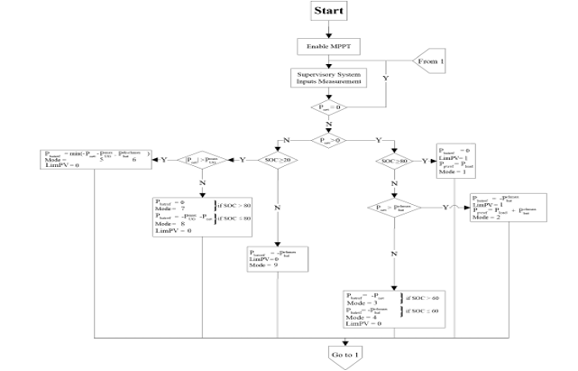Figure 17: EMS 3 flowchart

4. Simulation Results & Discussion

      The GCHRES performances under supervision of each EMS, are tested by simulation on MATLAB/SIMULINK, during a whole day of January. Simulation time are 24 Seconds within the logic of assigning a second to each hour. In order to test the system in all EMSs operating modes, the demand profile  for this month has been modified. However, the solar irradiation and temperature profiles have not been changed. The UG subscription power is fixed at -5kW, and the maximum injectable power, in grid injection limitation case is 1kW. Let’s remember that the maximum charging power of the battery is =-4.9kW, and its maximum discharging power is =4.6kW. The minimum and maximum battery state of charge SOC fixed at the battery sizing section are respectively  and   LimPV is the supervisory output that indicates the PVG control algorithm. If LimPV = 1 then the PVG is controlled by LPPT, otherwise, if LimPV = 0 then the PVG is controlled by MPPT. Note that peak hours run from 18h to 23h in January in Morocco. The adopted sampling time is s. Each simulation is divided into three time slots, and each time slot is divided into time intervals corresponding to the same operating mode (Opmodes): – 1^st time slot “From t=0s to t=10s”: Solar production is equal to zero =0, then begins to increase at t=8s, but insufficiently. This phase corresponds to insufficient PVG production ( <0). All EMSs are presenting the same results during this time slot, since their flowcharts are similar when <0. In order to avoid presenting the same results for many times, only one simulation will be carried out during this time slot, for all EMSs.  – 2^nd time slot “From t=10s to t=18s”: Solar production is quite high > 0). Sometimes it exceeds demand >0), and that is where the EMSs differ. In effect for the reversible/irreversible electromechanical metering case, if the power is injectable into the UG without limitation, the PVG operates globally in MPPT mode according to EMS 1. For the same metering cases discussed above, if the injectable power into the UG must be limited, PVG operates in LPPT mode in certain cases according to EMS 2. For digital metering case, according to EMS 3, the PVG operates also in LPPT mode in certain situations, to avoid injecting energy into UG. Situations where the PVG control switches toward LPPT are determined by the battery and the UG constraints. A specified demand profile has been dedicated for each EMS for testing their performances in their different operating modes.  – 3^rd time slot “From t=18s to t=24s”:  The system returns to an operating mode similar to the one on the first time slot, and in which all EMSs have a similar behavior according to their flowcharts. The system presents insufficient production from the PVG <0). Consequently, a single simulation will be adopted for all EMSs. The demand profiles used for simulating these EMSs at the different time slots are presented in Figure 18.

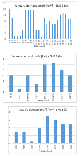Figure18: EMSs January demand profiles (a) EMS 1 whole day (b) EMS 2 between 10sec and 18sec (c) EMS 3 between 10sec and 18sec

4.1.  Energy Management Strategy 1 (EMS1)

 Time slot “From t=0s to t=10s”

The operating modes (OPmode) and the PVG limitation power decision (LimPV) are presented in Figure 19. Figure 20 presents the battery SOC evolution during this time slots. The net power  is presented in Figure 21, and the different system powers are all depicted in Figure 22.

Figure 23 shows the battery power  with its reference , and shows also the respect of the battery power constraints  and . UG power , respecting its constraint , is illustrated in Figure 24. It will be assumed that the battery has an initial SOC of 75%, due to its operation during the previous 24 hours, and in the aim to make the simulation as realistic as possible. According to Figure 20, the battery was sufficiently charged throughout this time slot  = 75% and  = 54.65%). Thus, the SOC constraint was respected, and therefore the battery had been operational throughout this time slots. From Figure 21,  < 0 throughout this time slot, and hence the system is on solar generation deficit. The PVG had worked under MPPT control throughout this simulation.

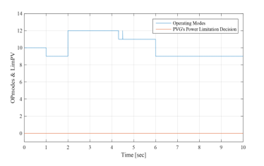Figure 19: Operating modes and PVG limitation decision between 0sec and 10sec (EMS 1)

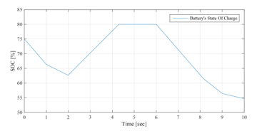Figure 20: Battery SOC evolution between 0sec and 10sec (EMS 1)

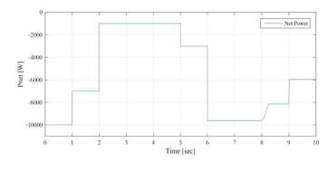Figure 21: Solar net power between 0sec and 10sec (EMS 1)

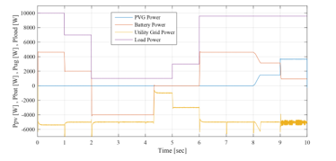Figure 22: PVG, battery, UG and load powers between 0sec and 10sec (EMS 1)

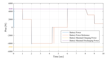Figure 23: Battery and battery reference powers between 0sec and 10sec (EMS1)

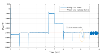Figure 24: UG power between 0sec and 10sec (EMS 1)

Opmode = 10 è from t=0s to t=1s: demand is excessively high ( 10kW) and slightly exceeds the power given by associating the UG with the battery at their maximum operating powers   4.6kW +  = 9.6kW < ). The battery performs its peak shaving function while respecting its constraint by not exceeding its maximum discharge power . The aim of this EMS is to continuously meet demand, while respecting the technical constraints related to the battery. Therefore, the UG is forced to slightly exceed its maximum power with a value of -0.4kW , in order to preserve internal circuits of the battery. This will rarely occur since in reality, late at night, demand is quite low. But as said previously, the purpose of modifying the demand profile is to test the performances of the GCHRES during the different EMS operation. This little overflow, which occurs rarely, will be acceptable since in return, the battery, considered as a highly vulnerable device, will be protected, and thus its lifespan will be extended. The SOC decreases rapidly as the battery discharges with its maximum power.

Opmode = 9 è from t=1s to t=2s & from t=6s to t=10s: On this time intervals, PVG/UG/battery combination is able to satisfy demand (  before t=8s thus ). Before t=8s, demand exceeds the UG maximum Power  and the latter constitutes the primary power source   , while the battery performs its peak shaving function. Its SOC decreases in function of the requested power from the battery (  ), which is lower than its maximum value . Around t=8s, sun begins to rise, and solar energy becomes the primary energy source destined to meet demand, but remains insufficient <0), since solar irradiation is too low at the first Hours following sunrise. The UG brings the deficit while not exceeding its maximum power   , then the battery is discharged in function of PVG+UG deficit ( , performing its peak shaving application. During this phases, the power requested by the battery is lower than previous phase (between t=0s and t=1s), which explains the SOC low decrease. A brief exceeding of the maximum power of the UG is noticed from t=8s to t=8.3s due to the MPPT control transient, which requires a little time for tracking the MPP, given that  before t=8s, hence the UG compensate this transient. It should be noticed that the transient lasts about 0.3, which is totally negligible in the real life operation of the system throughout the 24 hours of the day. Since it starts generating power, PVG operates in MPPT mode.

Opmode = 12 è from t=2s to t=4.3s: Demand is quite low, and UG can satisfy it alone without reaching its maximum power . As mentioned previously, all EMSs aim to charge the battery as soon as possible with the available source to get operational once peak shaving is requested. Therefore, the UG satisfies the demand, and the battery is charged by the difference between the maximum UG power and the demand . The battery charging power does not exceed its maximal value . In this time period, the UG power is always equal to its maximum . SOC increases according to the value of ( . At t=4.3s, the SOC reached its maximum ( , and the charging operation got stopped .

Opmode = 11 è from t=4.3s to t=6s: Demand does not exceed the UG maximum power ( . Since the battery SOC reaches its maximum , the charging process is no longer authorized . As a result, the UG is strained only to meet demand . The SOC remains stable at the value of 80%, and the battery power is equal to zero = 0).

 Time slot “From t=10s to t=18s”

     The operating modes (OPmode) and the PVG limitation power decision (LimPV) are presented in Figure 25. Since the injection into UG is not limited, the LPPT control is never activated (LimPV=0). Therefore, the PVG operates continuously in MPPT mode. Figure 26 presents the battery SOC evolution. The net power  is presented in Figure 27, and the different system powers are depicted together in Figure 28. Figure 29 shows the battery power  with its reference , and shows also the respect of the battery power constraints  and . In the beginning of this time slots, the battery  = 54.65%. From Figure 27,  > 0 between t=10s and t=15s, and <0 between t=15s and t=18s. Therefore, the system begins with a surplus of solar generation and then gets into deficit situation.

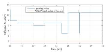 Figure 25: Operating modes and PVG limitation decision between 10sec and 18sec (EMS 1)

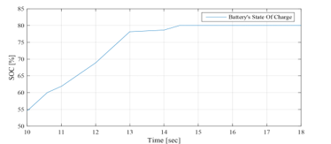 Figure 26: Battery SOC evolution between 10sec and 18sec (EMS 1)

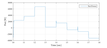 Figure 27: Solar net power between 10sec and 18sec (EMS 1)

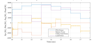Figure 28: PVG, battery, UG and load powers between 10sec and 18sec (EMS 1)

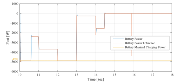 Figure 29: Battery and battery reference powers between 10sec and 18sec (EMS 1)

Opmode = 8 è from t=10s to t=10.6s: PVG power increases with solar irradiation increase. It is sufficient to satisfy the load demand but still less than battery maximum charging power < . This surplus is used to charge the battery, since its SOC is lower than its maximum value . And in order to ensure rapid charging of the battery (due to the SOC value inferior to 60%), aiming to obtain sufficient SOC for the next peak shaving request, the UG provides the necessary power, added to the surplus  , in order to charge the battery with its maximum power . Therefore, it is noticed that the SOC increases rapidly during this period.

Opmode = 7 è from t=10.6s to t=12s & From t=13s to t=14.3s: PVG is largely sufficient to satisfy the demand, but the surplus is still less than the battery maximum charging power . This surplus is used to charge the battery, since its SOC is lower than its maximum value ). The latter being quite high (SOC> 60%), the UG power is not requested ( , and the battery is charged only by the solar generation surplus  , which does not exceed the maximum charging power of the battery. Thus, its SOC increases, and its evolution depends on the value of . Since SOC reaches its maximum, the battery charging is no longer authorized ( at t = 14.3s).

Opmode = 6 è from t=12s to t=13s: PVG is largely sufficient to satisfy the demand and the surplus is greater than the battery maximum charging power > ). This is used to charge the battery with its maximum charging power , since its SOC is lower than its maximum limit . The remaining power is injected into the UG ( .

Opmode = 3 è from t=14.3s to t=15s: PVG is largely sufficient to satisfy the demand ( >0). As the battery had reached its maximum , charging operation is no longer authorized . The battery SOC remains stable at its maximum. The total solar generation surplus is injected into the UG .

Opmode = 11 è from t=15s to t=18s: The system return in the operating mode 11. Demand exceeds PVG production ( <0). The deficit being less than the UG maximum power , only the latter is requested to supports the PVG to meet demand . However, the battery which had reached its maximum state of charge  at t=15s, remains at rest  and its SOC stable at its maximum recommended.

 Time slot “From t=18s to t=24s”

     The operating modes (OPmode) and the PVG limitation power decision (LimPV) are presented in Figure 30. Figure 31 present the battery SOC Evolution during this time slots. The net power  is presented in Figure 32, and the different system power are depicted together in Figure 33. Figure 34 shows the battery power  with its reference , and shows also the respect of the battery power constraints  and . UG power , respecting its constraint , is illustrated in Figure 35. In the beginning of this time slots, the battery SOC is maximum recommended ( . At the evening, the PVG stops producing electricity and all demand will have to be met by the UG grid first, backed up by the battery performing the peak shaving. In effect, the UG contributes with its maximum power ), since the demand exceeds it ( . The battery provides the deficit (peak shaving), which is less than its maximum discharging power , according to the difference between the maximum UG power and the demand (  This lead to reduce the call of the UG during this time slot corresponding to peak hour interval in Morocco, reducing therefore the risks of grid congestion. The SOC is consequently in permanent decrease, reaching at the end of the day a value of 53%.

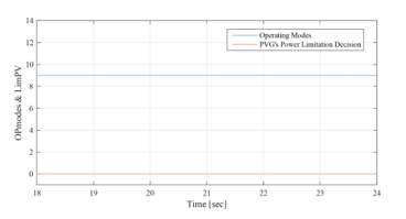Figure 30: Operating modes and PVG limitation decision between 18sec and 24sec (EMS 1)

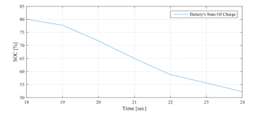Figure 31: Battery SOC evolution decision between 18sec and 24sec (EMS 1)

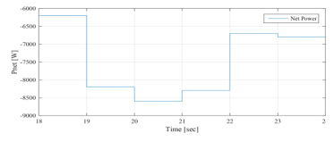 Figure 32: Solar net power between 18sec and 24sec (EMS 1)

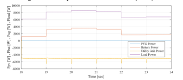 Figure 33: PVG, battery, UG and load powers between 18sec and 24sec (EMS1)

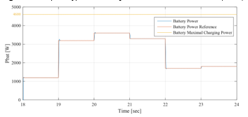 Figure 34: Battery and battery reference powers between 18sec and 24sec (EMS1)

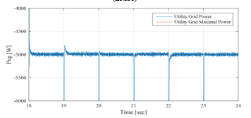 Figure 35: UG powers between 18sec and 24sec (EMS 1)

4.2.  Energy Management Strategy 2 (EMS2)

 Time slot “From t=10s to t=18s”

     As mentioned before, 1^st and 3^rd time slots is simulated only once and it represent the performances of the GCHRES supervised by each one of the three EMSs. Therefore, only the  time slot is simulated for EMS 2, and starts with the same conditions as those of the EMS 1. The operating modes (OPmode) and the PVG limitation power decision (LimPV) are presented in Figure 36. Figure 37 presents the battery SOC Evolution during this time slots. The net power is presented in Figure 38, and the different system powers are depicted together in Figure 39. Figure 40 shows the battery power  with its reference , and shows also the respect of the battery power constraints  and . The UG power, respecting its constraint , is illustrated in Figure 41. In this figure, it is shown that in case of injection into the UG, the power never exceeded 1kW, achieving consequently the purpose of keeping the UG voltage, bellow the maximum admissible voltage.  Figure 42 shows the PVG output power , and its reference  (when operating in LPPT). The PVG operating voltages (  are presented in Figure 43. From Figure 38, it is clear that  > 0 from t=10s to t=16s, and  < 0 from t=16s to t=18s. Therefore, the system begins with a surplus of solar generation and then gets into deficit situation.

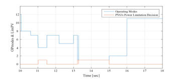Figure 36: Operating modes and PVG limitation decision between 10sec and 18sec (EMS 2)

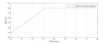Figure 37: Battery SOC evolution between 10sec and 18sec (EMS 2)

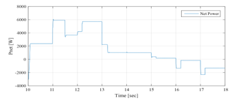Figure 38: Solar net power between 10sec and 18sec (EMS 2)

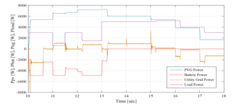 Figure 39: PVG, battery, UG and load powers between 10sec and 18sec (EMS 2)

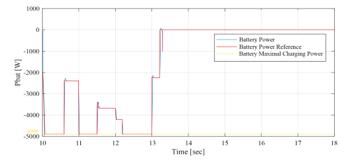Figure 40: Battery and battery reference powers between 10sec and 18sec (EMS2)

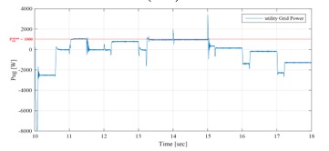 Figure 41: UG power between 10sec and 18sec (EMS 2)

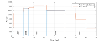Figure 42: PVG and PVG reference powers between 10sec and 18sec (EMS 2)

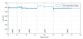Figure 43: PVG operating voltage between 10sec and 18sec (EMS 2)

Opmode = 8 è from t=10s to t=10.6s: PVG power increases with solar irradiation increase. It is sufficient to satisfy the load demand but still less than battery maximum charging power < . Hence, the PVG operates in MPPT mode. This surplus is used to charge the battery, since its SOC is lower than its maximum value . And in order to ensure rapid charging of the battery (due to the SOC value inferior to 60%) aiming to obtain sufficient SOC for the next peak shaving request, the UG provides the necessary power, added to the surplus  , in order to charge the battery with its maximum power . Therefore, it is noticed that the SOC increases rapidly during this period.

Opmode = 7 è from t=10.6s to t=11s & from t=11.5s to t=12.2s & from t=13s to t=13.2s:  PVG is largely sufficient to satisfy the demand, but the surplus is still less than the battery maximum charging power . Hence, the PVG operates under MPPT control. This surplus is used to charge the battery, since its SOC is lower than its maximum value ). The latter being quite high (SOC > 60%), the UG power is not requested ( , and the battery is charged only by the solar generation surplus  , which does not exceed the maximum charging power of the battery. Thus, the SOC increases and its evolution depends on the value of . Since SOC reaches its maximum recommended, the battery charging is no longer authorized ( at t = 13.2s).

 Opmode = 4 è from t=11s to t=11.5s: PVG is largely sufficient to satisfy demand, and the surplus 6kW is higher than the battery maximum charging power added to the UG maximum power injectable kW = 5.9kW ). Therefore, The LimPV supervisory output takes the value 1 in order to switch to the LPPT control of the PVG, whose output power  follows the reference  The PVG power is limited to the value kW+4.9kW+1 kW=6.5kW, and is reached by imposing the highest of the two voltages making it possible to reach this operating point, located in the right side of the MPP voltage on the ( , ) Curve. The SOC being less than its maximum value , the battery is charged via its maximum charging power ) and a power of 1kW is injected into the UG ).

Opmode = 5 è from t=12.2 to t=13 s: PVG is largely sufficient to satisfy demand. Surplus 5.71kW) is higher than battery maximum charging power but remain lower than the latter added to the UG maximum injectable power   1kW +  = 5.9kW). Therefore, the PVG operates under the control of the MPPT algorithm. The battery, whose SOC has not yet reached its maximum , charges via its maximum power ), and the remaining power ( =5.71kW–4.9 kW=0.81kW) is injected into the UG. Opmode = 1 è from t=13.2s to t=15s: PVG is highly sufficient to satisfy demand . Battery charging is no longer authorized ( since its SOC had reached its maximum value  at t=13.2s. As the injection into the grid is limited, The LimPV output took the value 1 to switch toward LPPT control. The PVG output power is limited to the value of 5kW+1kW=6kW, generated by the supervisory system, and a 1kW power was injected into the UG . SOC value is stable at its maximum value . As for time interval starting from t=11s and finishing at t=11.5s, the voltage imposed by the LPPT algorithm is the one higher than the MPP voltage. Opmode = 2 è from t=15s to t=16s: PVG is highly sufficient to satisfy demand . As the battery charging is no longer allowed ( ), the surplus is totally injected into the UG , since the maximum injectable power  is higher than the solar generation surplus . The PVG is to be controlled by MPPT.

Opmode = 11 è from t=16s to t=18s: Demand exceeds PVG production ( <0) and therefore the PVG is controlled by MPPT. The deficit being less than the UG maximum power , only the latter is requested to supports the PVG to meet demand . However, the battery which had reached its maximum state of charge  at t=15s, remains in rest  and its SOC stable at its maximum.

4.3.  Energy Management Strategy 3 (EMS3)

 Time slot “From t=10s to t=18s”

      The simulation starts with the same conditions as those of the EMS 1 and EMS 2 (  = 54.65%). The operating modes (OPmode) and the PVG limitation power decision (LimPV) are presented in Figure 44. Figure 45 presents the battery SOC Evolution during this time slots. The net power is presented in Figure 46, and the different system powers are depicted together in Figure 47. Figure 48 shows the battery power   with its reference , and shows also the respect of the battery power constraints  and . The UG power, respecting its constraint , is illustrated in Figure 49. It proves also that zero power was injected into the UG, avoiding thereby the occurring of an absurd increase of the subscriber energy bill. Figure 50 shows the PVG output power , and its reference  (when operating in LPPT mode). The PVG operating voltages  are presented in Figure 51. From Figure 46, it is clear that  > 0 from t=10s to t=14.3s, and  < 0 from t=14.3s to t=18s. Therefore, the system begin with a surplus of solar generation and then gets into deficit situation.

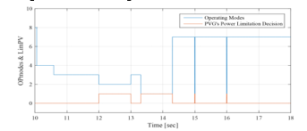Figure 44: Operating modes and PVG limitation decision between 10sec and 18sec (EMS 3)

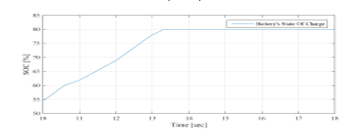Figure 45: Battery SOC evolution between 10sec and 18sec (EMS 3)

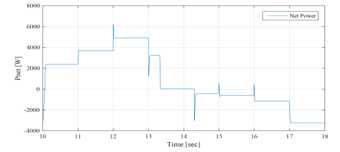Figure 46: Solar net power between 10sec and 18sec (EMS 3)

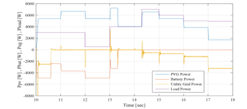Figure 47: PVG, battery, UG and load powers between 10sec and 18sec (EMS 3)

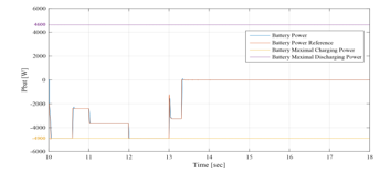Figure 48: Battery and battery reference powers between 10sec and 18sec (EMS3)

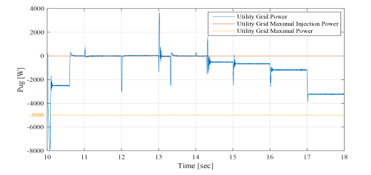Figure 49: UG power between 10sec and 18sec (EMS 3)

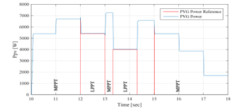Figure 50: PVG and PVG reference powers between 10sec and 18sec (EMS 3)

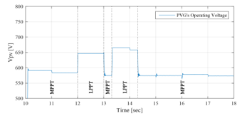Figure 51: PVG operating voltage between 10sec and 18sec (EMS 3)

Opmode = 4 è from t=10s to t=10.6 s: PVG generation increases with solar irradiation increase. It is sufficient to satisfy the load demand but still less than battery maximum charging power < . Hence, the PVG operates under MPPT control. This surplus is used to charge the battery, since its SOC is lower than its maximum value . And in order to ensure rapid charging of the battery (due to the SOC value inferior to 60%) aiming to obtain sufficient SOC for the next peak shaving request, the UG provides the necessary power, added to the surplus  , in order to charge the battery with its maximum power . Therefore, it is noticed that the SOC increases rapidly during this period.

Opmode = 3 è from t=10.6 to t=12 s & from t=13 to t=13.3 s:  PVG is highly sufficient to satisfy the demand, but the surplus is still less than the battery maximum charging power < . Hence, the PVG operates under MPPT control. This surplus is used to charge the battery, since its SOC is still lower than it maximum value . The latter being quite high (SOC> 60%), the UG power is not requested ( , and the battery is charged only with solar generation surplus  , which does not exceed the maximum charging power of the battery. Thus, we notice that the SOC increases, and its evolution depends on the value of . Since SOC reached its maximum limit , the battery charging is no longer authorized ( at t = 13.3s).

Opmode = 2 è from t=12s to t=13s: PVG is largely sufficient to satisfy the demand, and the surplus is greater than the maximum charging power of the battery > . The SOC being less than it maximum value , the battery starts charging with its maximum charging power . Since injection into UG is not authorized , The LimPV output takes the value 1 in order to switch to LPPT control. The PVG output power is limited to the value of 0.5kW+ 5.4kW, calculated by the supervisor. The SOC increases rapidly as the battery charges with its maximum charging power. The voltage imposed by the LPPT algorithm is the one higher than the MPP voltage.

Opmode = 1 è from t=13.3s to t=14.3s: PVG is satisfying the demand (  > 0) and the battery SOC has reached its maximum value , thus the battery can no longer be charged ( . As the injection into the UG is not authorized ( , the PVG is controlled by LPPT. The LimPV output takes the value 1 to switch toward the LPPT control. The PVG reference power set by the supervisor is equal to 4kW. The battery remains at rest and its SOC equal to its maximum recommended  , and the voltage imposed by the LPPT algorithm is the one higher than the MPP voltage.

Opmode = 7 è from t=14.3s to t=18s: Demand exceeds PVG production ( <0), therefore the PVG is controlled by MPPT control. The deficit being less than the UG maximum power , only the latter is requested to supports the PVG to meet demand . The battery whose SOC is equal to its maximum ,  remains at rest .

4.4.  Overall System Results

     Figure 52 shows that the overall system real power is equal to zero, which proves the performances of the GCHRES in terms of stability and power quality. Line to line voltages of the load is altered if the system contains real power [24]. From Figure 53, it is seen that the DC- bus voltage is inside standard limits [25], and Figure 54 shows the zero reactive power exchange between the ASC and the CCP. It should be noticed that the transients present in some figures as the ones corresponding to the UG power and the overall system net power, are due to the loads switching via circuit breakers in MATLAB/SIMULINK, and last no longer than tenth of second, which is negligible in the case of the real operation of the system throughout the 24 hours of the day.

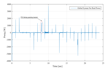Figure 52: Overall system real power (simulation for EMS 1)

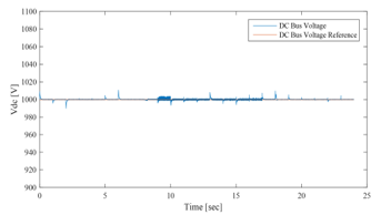Figure 53: DC-Bus voltage vs reference (simulation for EMS 1)

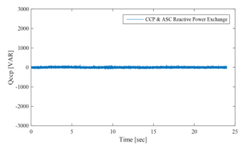Figure 54: Reactive power exchange between ASC and CCP (simulation for EMS1)

5. Conclusion

     This paper presents three novels energy management strategies controlling the power flows within a GCHRES. The proposed EMSs differ according to the UG metering types. They have for common purpose to continuously meet the variable demand of the load for the whole 24 Hours of the day. They aim also to avoid the battery lifespan reducing, and to reduce the monthly energy bill of the UG subscriber through battery peak shaving application. The dynamic behaviours of the proposed GCHRES, under the supervision of these several EMSs, are tested under real weather data and variable load demand profiles. The effectiveness of the developed system in terms of demand meeting, DC-Bus voltage regulation, overall system stability, power quality, and element constraints respecting, is confirmed by simulation in MATLAB/SIMULINK.

Conflict of Interest

The authors declare no conflict of interest.

1. K. H. Hussein, I. Muta, T. Hshino and M. Osakada, “Maximum photovoltaic power tracking: an algorithm for rapidly changing atmospheric conditions,” IEE Proceedings -Generation, Transmission and Distribution, 142(1), 59–64, January 1995, doi:10.1049/ip-gtd:19951577.
2. T. Wu, C. Chang, and Y. Chen, “A fuzzy – logic controlled single-stage converter for PV-powered lighting system application,” IEEE Transactions on Industrial Electronics, 47(2), 287–296, April 2000, doi:10.1109/41.836344.
3. C. Zhang, D. Zhao, J. Wang, and G. Chen, “A modified MPPT method with variable perturbation step for photovoltaic system,” in 2009 IEEE 6th International Power Electronics and Motion Control Conference, 2096–2099, 2009, doi:10.1109/ipemc.2009.5157744.
4. R. Faranda, S. Leva, V. Maugeri, “MPPT techniques for PV systems: energetic and cost comparison,” in 2008 IEEE Power and Energy Society General Meeting – Conversion and Delivery of Electrical Energy in the 21st Century, 2008, doi:10.1109/pes.2008.4596156.
5. Patcharaprakiti N., Premrudeepreechacharn S., Sriuthaisiriwong Y, “Maximum power point tracking using adaptive fuzzy logic control for grid connected photovoltaic system,” Renewable Energy, 30(11), 1771–1788, 2005, doi:10.1016/j.renene.2004.11.018.
6. M. Dharif, Modélisation de l’intégration de l’énergie photovoltaïque au réseau électrique national, Ph. D Thesis, Cadi Ayyad University -Sciences and Technology Faculty of Marrakech, 2016.
7. S.-I. Go, S.-J. Ahn, J.-H. Choi, W.-W. Jung, S.-Y. Yun and I.-K. Song, “Simulation and Analysis of Existing MPPT Control Methods in a PV Generation System,” Journal of International Council on Electrical Engineering, 1(4), 446–451, 2011, doi:10.5370/jicee.2011.1.4.446.
8. N. Femia, G. Petrone, G. Spagnuolo and M. Vitelli, “Optimizing sampling rate of P&O MPPT technique,” in 2004 IEEE 35th Annual Power Electronics Specialists Conference, 3, 1945-1949, June 2004, doi:10.1109/pesc.2004.1355415.
9. X. Liu, L. A. C. Lopez, “An improved perturbation and observation maximum power point tracking algorithm for PV arrays,” in 2004 IEEE 35th Annual Power Electronics Specialists Conference, 3, 2005-2010, June 2004, doi:10.1109/pesc.2004.1355425.
10. A. Bennouna, “Autoproduction d’électricité-Pour qui est fait le Projet de Loi en gestation ?,” chantiers du maroc, 2 December 2020, https://chantiersdumaroc.ma/btp-qui-bouge/dossiers/autoproduction-delectricite-renouvelable-la-loi-en-gestation/.
11. European Parliament, “Outlook of Energy Storage Technologies”, European Parliament’s committee on Industry, Research and Energy (ITRE), 2008,IP/A/ITRE/FWC/2006-087/Lot4/C1/SC2. http://www.storiesproject.eu/docs/study_energy_storage_final.pdf.
12. Y. Riffonneau, Gestion des flux énergétiques dans un système photovoltaique avec stockage connecté au réseau, Ph. D Thesis, Grenoble Alpes University, 2009.
13. A. Bennouna, “Produire son électricité solaire au Maroc, c’est possible et peut être rentable… malgrès tout !,” EcoActu, 30 March 2020, https://www.ecoactu.ma/produire-son-electricite-solaire/.
14. A. Guichi, A. Talha, EM. Berkouk, S. Mekhilef, “Energy Management and Performance Evaluation of Grid Connected PV-Battery Hybrid System with Inherent Control Scheme,” Sustainable Cities and Society, 41, 490–504, 2018, doi:10.1016/j.scs.2018.05.026.
15. P.B.S. Kiran, Limited Power Control of a Grid Connected Photovoltaic System, Ph. D Thesis, Indian Institute of Technology Gandhinagar, 2015.
16. A. Bouharchouch, EM. Berkouk, T. Ghennam, “Control and Energy Management of a Grid Connected Hybrid Energy System PV-Wind with Battery Energy Storage for Residential Applications,” in 2013 Eighth International Conference and Exhibition on Ecological Vehicles and Renewable Energies (EVER), 2013, doi:10.1109/ever.2013.6521525.
17. J. Labbé, L’hydrogène électrolytique comme moyen de stockage d’électricité pour systèmes photovoltaiques isolés, Ph. D Thesis, Paris Mining School, 2006.
18. A. Dekkiche, Modèle de batterie générique et estimation de l’état de charge, Master in Electronic, Superior Technology school, Quebec University, 2008.
19. O. Tremblay, L. A. Dessaint, A. I. Dekkiche, “A Generic Battery Model for the Dynamic Simulation of Hybrid Electric Vehicles,” in 2007 IEEE Vehicle Power and Propulsion Conference, 284-289, 2007, doi:10.1109/vppc.2007.4544139.
20. R. A. Jackey, “A simple, Effective Lead-Acid Battery Modelling Process for Electrical System Component Selection,” SAE International, 116(7), 219–227, 2007, doi: https://doi.org/10.4271/2007-01-0778.
21. M. Ceraolo, “New dynamical models of Lead-Acid batteries,” IEEE Transactions on Powers Systems, 15(4), 1184–1190, 2000, doi:10.1109/59.898088.
22. SimPowerSystems TM Reference, Hydro-Québec/the Math Workds, Inc., Natick, MA, 2010.
23. European Commission website “ec.europa.eu”, European Commission > EU Sciences Hub > PVGIS > Outils Interactifs, lattest update 15 October 2019, https://re.jrc.ec.europa.eu/pvg_tools/fr/#MR
24. K. Tariq, H.S. Zulqadar, “Energy Management simulation of Photovoltaic/Hydrogen/Battery Hybrid Power System,” Advances in Science, Technology and Engineering Systems Journal, 1(2), 11–18, 2016, doi:10.25046/aj010203.
25. “IEEE Standard for Interconnecting Distributed Resources with Electric Power Systems,” IEEE Std 1547-2003, 2003.

(Click Here)