1. Introduction

This paper is an extension of a work originally presented in the First International Conference on Cyber Management and Engineering (CyMaEn`21) [1].

During more than 300 years, there were only two kinds of movements known in simple dynamical systems: the uniform and the accelerated movements. Maxwell and Poincare were among the minority of scientists who disagreed with those facts. It was only in the last quarter of the 20^th century that the third kind of movement appeared: chaos [2].

The existence of dynamics and nonlinearity in the brain has been the topic of numerous research investigations since the 1980s. In [3], it was revealed in neurosciences that the activity of the olfactory bulb of rabbits is chaotic and, at any time, it may switch to any perceptual state (or attractor). In fact, the experimentations assessed that when rabbits inhale an odorant, their Electroencephalograms (EEGs) display gamma oscillations, signals in a high-frequency range [4, 5]. The odor information represents then an aperiodic pattern of neural activity that could be recognized whenever there was a new odor in the environment of after a session of training.

Furthermore, during the same period of Freeman’s research, other works figured out the existence of chaos in the temporal structure of the firing patterns of squid axons, of invertebrate pacemaker cells, and in temporal patterns of some brain disorders such as schizophrenia and human epileptic EEGs [4-7]. Moreover, in red blood cells, chaotic dynamics of sinusoidal flow were determined by 0-1 test. In fact, numerous simulations identified the existence of chaotic dynamics and complexity in the sinusoidal blood flow [8]. In addition, the exploration of dreaming through the application of concepts from chaos theory to human brain activity during Rapid-Eye-Movement state (REM-state) sleep/dreaming proved that chaos is on the flow of thoughts and imagery in the human mind [8-10]. Finally, chaos is ubiquitous in the brain operations and cognitions according to cognitive sciences, linguistics, psychology, philosophy, medical sciences, and human development [11-15]. The later issues are still addressed in depth in the context of research on the complex systems, to which the brain obviously belongs. This is at this level that the ultimate goal of AI has to be considered. Indeed, creating a machine exhibiting human-like behavior or intelligence, cannot be, with keeping the chaos properties aside.

Moreover, being an offshoot of Artificial Intelligence (AI) paradigms, pattern recognition techniques focus on the identification of regularities in data in an automated process [16]. It is worth noting the fact that, pattern recognition is a cognitive functionality in the brain. In fact, in real life, human beings are capable of recognizing and recalling patterns of different natures and forms (not necessarily perfect patterns) and in different conditions, naturally without significant effort.  An intelligent pattern recognition system must thus include brain properties, such as, the presence of chaos.

 Furthermore, ANNs represent a discipline of AI that has successfully been applied on different nature of pattern recognition problems. In fact, ANNs models were employed for data compression, data classification, data clustering, feature extraction, etc. Data classification is particularly one of the most active search and application fields in connectionism [16-18].  Consequently, ANN approaches encompasses potential techniques to face pattern recognition problems.

Several works can be noticed in the literature, that focus on the construction of ANN models that implement NDS properties [19-23]. Those proposed models are challenging the classical kinds of ANNs in terms of biological plausibility [24-28], and in some cases, even in terms of computational efficacy of the model [29-32]. Except that, most of the proposed models were developed including the stabilities of attractors with no attention to the ongoing instabilities. The present work shows the chaos potentials in a recurrent ANN model in comparison with two other conventional ANN models. The potentials are such as a perfect pattern recognition accuracy and an excellent resilience to noise. In addition, the model proposed in this paper faces two aspects in the biological plausibility formerly mentioned; the resilience to noise, and as a matter of fact that chaotic properties are actually present in the brain.

In the present work, three different ANN models are investigated as pattern recognition systems in two different real-life classification domains: substance identification and breast cancer identification.

1.1.  Substance identification

Sensing technology encloses various instrumentation techniques for variable characterization in diverse aspects of human life [33]. From a hybridization of chemical and physical measurement devices, results the construction of biosensors. Those devices are capable of converting a chemical or physical characteristic of a particular analyte into a measurable signal [34]. Those devices offer a great potential for several integrated applications for rapid and low-cost measurement and were widely used in contrastive scientific practice, certainly owing to their remarkable outcome [33-39]. Biosensors were developed throughout various applications and principally put an accent on the construction of sensing components and transducers. Those applications fall under a multiple substance analysis for diagnosis [40-44], and estimations [45-48].

      The technology of sensor devices led to remarkable achievements that are undeniable. Except that, it remains important in any sensing process to create a steady and precise pattern recognition model admitted to the sensory system for substance detection [33]. The raw data that are collected from the sensor need to be analyzed. For that purpose, and to offer a complete integrated instrument, the classical method has suggested incorporating optical filters to the basic sensor, also, the use of statistical and threshold-value based techniques for data processing. Recent researches offer a potential and more efficient alternative: the use of AI paradigms. Plenty of applications can be found in the literature that use these pattern recognition methods for substance detection such like, Decision Trees [38], random forest [34, 43], K Nearest Neighbor [34, 40, 42], Support Vector Machine (SVM) [40-43], and ANNs [36-47].

The authors use in [47] a biochemical sensor to acquire fluorescence measurements from a variety of substances at different concentrations. The sensor prototypes utilized Light Emitting Diodes (LEDs) as excitation sources, as detailed in [47], and LEDs and/or photodiodes as photodetectors.

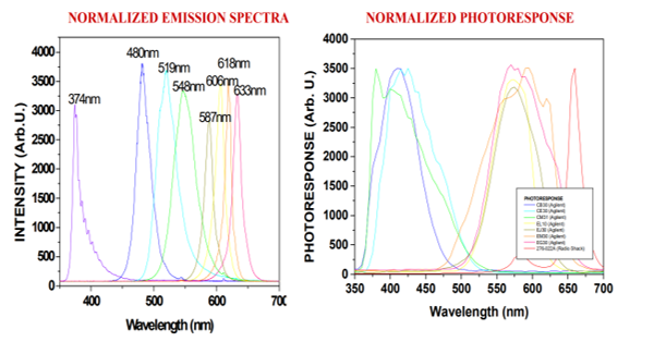
Figure 1: Sample mission and photo response spectra of the color LEDs [47]

Basically, the excitation light procured an interaction with the tested analyte of various aspects such as fluorescence, reflection, absorption, and scattering in a synchronous manner. The resulting light was quantified by the photodetectors having distinct spectral sensitivities. The LEDs were excited synchronously, one at a time, detecting the resultant fluorescence with the remaining LEDs. That was the process followed to collect an amount of data for each analyte at a specific concentration .This process generated a data collection that characterizes a singular spectral signature for a compound at a specific concentration, as illustrated in Figure 1. That process was repeated for all components at different concentrations. Then, after detecting and amplifying the data with a multi-wavelength sensor front end, they are used to train the ANN and, upon satisfactory training, the network is assigned to the identification of other data collected by the biosensor. The ability to determine very low substance concentration levels using the ANN dramatically increases the specificity of the biochemical sensor.

The focus of classification techniques is, for given input patterns, to detect target classes, determined to define a particular substance concentration pairs. In this context, the authors in [47] developed a MultiLayered neural network, that was trained with the collected data from the biosensor, to process the classification phase on data reserved to test the network. The topology of the network model is basically a Multi-Layered Neural Network (MLNN) which consists of two hidden layers with 56 processing neurons for each layer, and a single output neuron. The RProp algorithm was employed as a learning rule on the network to process the training phase. The learning algorithm in multilayered network models consists basically of two phases. At the beginning, an input pattern is randomly selected from the training dataset and is assigned to the input layer of the ANN. Then, the network propagates that pattern from layer to layer until a corresponding output pattern is computed by the output layer. In case there is a difference between the resulting pattern and the desired output, the error is estimated and then propagated in the opposite direction through the network, from the output to the input layers. In the meanwhile, the weights’ values are readjusted, as the error value is propagated backward [16].

In [47], the authors developed the MLNN to detect four fluorescent organic compounds at different concentrations, as one can notice on Table 1. The resulting performance attests a good classification capacity of the network, reaching more than 94% of perfect analyte detection. The error curves for both the training and the recall phases are plotted bellow in Figure 2.

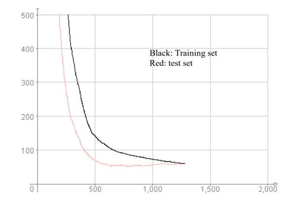
Figure 2: Sum-of-Squares classification error curves versus the number of cycles for the 56-56-56-1 MLNN topology.

Dealing with the same substance identification problem, the authors in [48] developed an evolutionary AI approach, based on Particle Swarm Optimization (PSO), viewing the detection problem as an optimized search. Indeed, the same datasets used in [47] were employed in the experimental set-up. The obtained results with the PSO model enhanced the recognition accuracy reaching 98% of exactitude.

The results of the latter two works and the same data collection were reserved in the present work, with the aim of trying to enhance even more the recognition rates obtained, by incorporating the properties of chaos in ANN models. We investigate a BAM and a CBAM recurrent models to process fluorescence data for the substance identification task.

1.2.  Breast cancer detection

Cancer is a disease that might attack numerous human organs. A scourge that continues spreading all over the world with alarming new statistics each year. Statistics report that, breast cancer is the 2^nd dangerous disease all over the world, in fact, the rate of mortality from this disease is overwhelming.

The WHO (World Health Organization), states that breast cancer affects more than 2 million women every one year across-the-board [49, 50]. In 2020, 2.3 million women were diagnosed with breast cancer and globally 15% of all death among women from cancer was from breast cancer disease. An early diagnosis of the disease, increases the chances of survival for the patient.

The main purpose of medical diagnosis aid systems for breast cancer disease is the detection of non-cancerous and cancerous tumors [49-53]. The only valid prevention approach for breast cancer disease remains the early diagnosis [54-56]. In the 1980s, in developed countries, with the establishment of early detection protocols and a set of treatment processes generate enhancements in survival rates. For a prevention purposes, the National Breast Cancer Foundation (NBCF) prescribe a mammogram once a year for women that are over 40 years old.

Technologies based on AI paradigms are getting more accurate and reliable results than conventional ones. AI tools such as pattern recognition techniques [49, 51, 53, 54, 55, 56], are estimated for being of great help in the medical diagnosis aid field. In fact, as part of breast cancer detection, doctors need to be able to differentiate between categories of tumors through a reliable procedure of examination. Specialists assess the fact that tumors’ diagnosis is a task that is considered to be very hard to accomplish. It is thus crucial to diagnose breast cancers in an automated manner to overcome that difficulty.

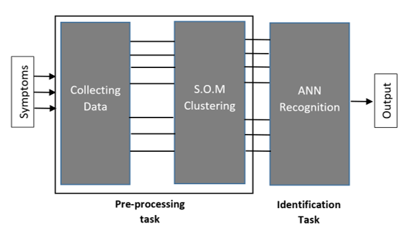
Figure 3: ANN for medical diagnosis aid system

In the field of breast cancer detection, numerous paradigms were employed to construct medical diagnosis aid systems. Those techniques use pattern recognition tools as Random forest [49-55], K-Nearest-Neighbor [52, 54], Logistic regression [51, 53], Naïve Bayes [49, 52, 53, 56], Decision Tree [49, 51-55]; not only but also ANN models [49-55], in particular, Support Vector Machines (SVM), Multi-Layer Neural Networks, Convolutional Neural Networks, or BAM neural network model. All those techniques have the same aim: the automation of breast cancer identification to assist medical diagnosis protocols.

As for the first pattern recognition task, the substance identification problem, the same three different ANN models are used in this work to face a breast cancer identification problem, such as, a MLNN, a BAM and a CBAM model.  Indeed, a different real-life pattern recognition problem is investigated with a different dataset to highlight the potential of chaos in an ANN model’s performance. The proposed ANN models are operating as breast cancer diagnosis aid systems according to the process shown in Figure 3. First, symptoms are collected from the diagnosed patients, thereby creating a raw database. Subsequently, raw data undergoes a preprocessing phase before being assigned to the ANN model for the identification phase. The preprocessing phase is detailed in the Data Acquisition section.

The rest of this paper is organized as follows. Section 2 proposes briefly an overview about models theory. Section 3 defines the properties and the pre-processing methods used on the two different datasets employed in the experimental set up, such as, the fluorescence based measurements and the breast cancer dataset. Section 4 presents the different parameters’ details and implementations’ descriptions of the developed ANN models with their respective results. The obtained results are discussed in the last section, the conclusion.

2. Theory of Models

Among the various AI techniques applied in pattern recognition problems, connectionist approaches proved their good ability to process classification, which represents the most active field in the research on ANNs [16, 18, 57]. We present in the rest of this section an overview of research works employing multilayered neural network models and memory-based ones. The kind of ANN models that we are about to present in this paper.

2.1.  Multi-Layered Neural Network (MLNN)

The MLNN is built in a multilayer Perceptron fashion. The architecture of such a model is composed of an input layer, one or more hidden layers of computing neurons, and an output layer generating an output pattern corresponding to the input assigned formerly to the network [18]. The MLNN performs a supervised learning. In addition, most of MLNNs processes their learning phase according to the basis of the pioneer backpropagation (Backprop) algorithm or one of its variants. In fact, an error is calculated according to the difference between an actual and a desired output patterns, which is propagated backward again through the network layers and the values of the weights are then updated to reduce it [16].

Basically, the backpropagation algorithm represents a chain rule to estimate the effect of each weight value in the network according to an arbitrary error-function [58]. Once all the weights of the connections are computed, the purpose is to make the error value as small as possible through an error-function. The commonly used error-function is the simple gradient descent including a learning rate parameter. The choice of that parameter has a considerable impact on the number of learning epochs needed for the ANN to converge. On the one hand, the smaller is the learning parameter the greater is the number of learning cycles. On the other, under a large value of the learning rate, the network risks to generate oscillation, which makes difficult to diminish the error value.

Given the limits of the classical Backpropagation rule, it has gone through several improved versions [16, 18, 58, 59], among which, introducing a momentum-term. A parameter that was supposed to make the learning algorithm more stable and the learning convergence quicker. However, it turns out experimentally that the optimal value of the momentum parameter is equally problem dependent as the learning rate, and finally, no general improvement can be carried out.

Later, numerous algorithms were proposed to face the problem of appropriate update of the weight values by using an adaptation parameter in the training epochs. That parameter is used actually to estimate the weight-step. The adaptation algorithms are  approximately grouped into two classes, local and global rules [58]. On the one hand, local adaptation rules employ the partial derivative to adjust weight-specific parameters. On the other hand, global ones employ the information concerning the state of the whole ANN model, meaning, it uses the orientation of the previous weight-step, to update global parameters. Basically, the local rules fit better the conception of learning in ANNs. Again, the adaptive enhanced version of the Backpropagation algorithm has certain limitations. Concretely, the impact of the chosen value of the adapted learning parameter is very sensitive to the partial derivative [16, 18, 58].

Finally, the weaknesses of all the aforementioned backpropagation variants took over the  conception of the Rprop. The fact that this algorithm updates the size of the weight-update directly and without taking into account the partial derivative’s size, keeps the system away from the ‘blurred adaptivity’ phenomenon. All the modified verisons of the backpropagation algorithm have the aim to accelerate the neural network convergence, and through various experimentations, the Rprop have proven to be more useful than the others. The Rprop learning scheme offers a great efficacy compared to the classical backpropagation algorithm and its above-mentioned modifications [58]. Basically, that learning rule processes the weight-step adaptation according to a local gradient information. In addition, the contribution made by the Rprop rule is that, the introduction of an individual update-value for each weight avoids the effort of adaptation to be blurred by the gradient behavior. Basically, the individual update-value determines the size of the weight-update. The value of the update parameter is estimated while the training is processed on the network, and that estimation is based on its error-function local information.

Through a set of experimentations on several MLNN models [47], the global error performance of the MLNN employing the RProp algorithm was the smallest. In addition, the speed of convergence of the model was the quickest one. Consequently, the resilient backpropagation  is implemented in the learning phase for the MLNN model in the present work. Apart from that, the sigmoid function [59] is employed as the neuron output function of the multilayered model.

2.2.  Bidirectional Associative Memory (BAM)

The first ANN model offering a learning  process operating in a heteroassociative scheme, was proposed in the 1970s [19]. That ANN was designed with a focus on constructing a formal system that demonstrates the way that brain associates different patterns.

In fact, when training the brain perceive something (input pattern), another one is recalled (output pattern, or a category). The pioneer memory-based ANN model is linear [19], whether through its training rule or its the unit activation function. That in fact limits the recall capacity of the network, especially in case correlation occurs in input patterns. That weakness of the model has pushed the research on the field to evolve towards the construction of recurrent auto-associative and interpolative models of memory that includes nonlinearity [20]. The later models generate dynamic functionalities through a nonlinear output feedback function. That function nonlinearity offers to the system the possibility to converge to stable fixed-points. Consequently, if the networks learned training patterns in correspondence with given fixed-point attractors, it would be capable of recalling them despite the presence of noise in data. The author in [60], used those characteristics to incorporate the nonlinear feedback of the Hopfield model to a hetero-associative memory model. Finally, the BAM came up, a new kind of brain-inspired connectionist models.

A Multilayered ANN model has different functionalities from a memory-based ANN model. Instead of propagating the signal in a layer-by-layer fashion from the input layer to output layer, the BAM consists of generating feedback loops from its output to its inputs; in fact, this model has a recurrent topology [18]. In addition, the learning process in memory-based ANN models are a brain-inspired artificial approach. Indeed, that learning process allows to develop attractors for each pattern since the recurrent architecture offers the ability of feedback connections [21]. Furthermore, learning with BAMs demonstrates a remarkable stability and adaptability against noise and a great capacity of generalization. The memory-based model has also exhibited a great potential for pattern recognition especially given its capacity to be trained under a supervised or an unsupervised scheme. The Hebbian rule is the common learning algorithm used for the unsupervised trainings in the BAM models [16]. If two units in the network are activated in a simultaneous way on either side of a connection, the corresponding weight is then increased. Otherwise, if two units in the BAM are activated in an asynchronous way on either side of a connection, the corresponding weight is thus decreased. Concretely that is the Hebb’s law basis. Being the fact that the Hebbian learning consists of an unsupervised learning, the process is local to the network and is performed independently of any external interaction.

The BAM training is originally performed with a classical Hebb’s law [16, 20]. Because of its multiple limitations, among which, pattern-correlation, there were numerous enhanced versions of the hebbian learning principle. The first memory-based model employed a nonlinear activation function (the Signum function) in the recall phase. Again, the latter learning rule had some limitations such as it is accomplished offline and the network is limited to bipolar/binary input patterns. In addition to, the BAM generates numerous inaccurate attractors and its memorization aptitude is limited.

To confront those limits, the learning algorithm was modified with the use of a projection matrix following the principle based on least mean squared error minimization. Other alternatives were put forward in the literature tempting to enhance the learning algorithm behaviors. In fact, the proposed models tried to overcome the classical learning rule by increasing the model’s storage capacity and his performance, but also by reducing the number of inaccurate states. Unfortunately, most of the proposed processes increases the neural network complexity [20].

In the present work, the authors use a BAM model that allows either an offline or an online learning of the patterns, and most of all, a model that is not limited to memorize binary or bipolar patterns. Indeed, the memory-based ANN model has to be capable of learning real-valued to deal with both of our real-life problems, substance identification and breast cancer detection. In the present work, the learning rule used in the BAM model is derived from the Hebbian/anti-Hebbian rule detailed in [43, 44].

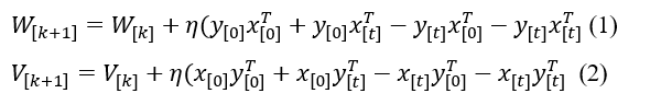
W and V in equations (1) and (2) are the weight matrices for both network directions, x_[0] and y_[0] are the initial inputs to be associated. The variable η represents the training parameter, whole k represents the number of learning cycles. Through x_[t] and y_[t], a feedback from a nonlinear activation function is included in the learning algorithm; which offers to the network the ability to learn online and then contributes to the convergence of the BAM’s behavior. Given those particularities, we opt to develop this learning function on the BAM model in the present work.

It is worth noting that, the cubic map detailed in [20, 22], is used as the unit output function of the memory-based model. The cubic map is employed for the BAM model under a non-chaotic mode, as detailed in section IV.

The training process of the BAM was performed under the basis of the following algorithm:

1)       Selecting randomly a pattern pair from the learning dataset;

2)       Computing X_t and Y_t according to the output function employed (Cubic-map);

3)       Computing the adjusted values of the weight matrix  according to (1) and (2);

4)       Reiteration of steps 1) to 3) until the weight marix converges;

This same learning rule is used further in the third ANN developed model, the C-BAM.

2.3.  Chaotic Bidirectional Associative Memory (C-BAM)

Since chaotic patterns were found in the brain [11, 12, 13, 14, 24, 25], numerous research works were proposed in the literature, tempting to include dynamic properties in ANN models. It must be noted that, time and change are the two properties that particularly defines the impressive properties of the NDS approach. As a result, those proposed NDS-based models are confronting the classical doctrines on brain functionalities and most of the theories that were assessed since the inception of neuroscience and cognitive sciences. This comes up with, challenging also the disciplines that focus on the construction of brain-inspired models such like artificial intelligence, and specifically ANNs paradigms.

 Furthermore, most of proposed models are of a computational nature and leave dynamic principles aside. Moreover, concerning the models that encompasses NDS characteristics, only fixed points are taken into account to store and retrieve information. As a result, characteristics of the NDS approach are kept aside [46, 50]. Basically, perceived as a nuisance, chaos is, most of the time, excluded from the models.

The main purpose in the construction of brain-inspired AI models, particularly ANNs; cannot however ignore principles of nonlinear dynamical systems.

Moreover, in spite the various existing models in connectionism, not all those models are applicable to include NDS properties. Indeed, memory-based models such as BAMs offer the ability to develop nonlinear and dynamic behaviors. In fact, their recurrent architecture offers characteristics that allow an ANN model to generate oscillations [20, 21, 22, 23, 24, 25].

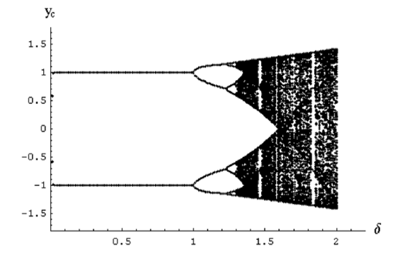
Figure 4: Bifurcation diagram of the cubic map [20].

The parameters employed in the CBAM model are as follows: the learning rule employed in the former BAM model, derived from the Hebbian/antiHebbian algorithm; also, the BAM’s topology is kept the same; and concerning the output function, 23 chaotic maps (including the former cubic-map) operating in a chaotic mode are used after training, at the recall phase.

Chaotic maps characteristics

We test a set of 22 chaotic function defined in detail in [2, 61, 62, 63, 64, 65], among which, the Spikin maps family, the Tent maps, the Mira group, the Bernoulli map, and the Henon map. The last map is the one that completes the CBAM model’s performance to perfect, at performing both the substance identification task and the breast cancer identification problem, as detailed further in this paper in the Experimentation section.

The 23rd function is the same cubic map used in the former BAM model, except that we set its parameters this time so that it can work in a chaotic mode. The function parameters are set according to its bifurcation diagram in the Figure 4, as detailed further in section IV. As one can notice, the process is capable of leading the system to stable attractors for value , although an aperiodic behavior can occur when the parameter value exceeds 1, and then, switching the system into a chaotic phase (black areas in the bifurcation diagram). The 23 output functions tested on the CBAM model are listed in Table 2.

The Henon map

This function is detailed in [2] as follows:

The Henon map has to inputs, such as x and y, and two outputs, the new values of x and y [2]. The use of the control parameters’ values α = 1.28 and β = -0.3, we notice that the orbit converges to a 2-period attractor (as shown in Figure 5), when at the value α=1.4 the attractor becomes fractal [2].

Table 1: The performances of the CBAM with the 23 maps, the BAM and the MLNN model.

ANN Model	Breast Cancer Recognition	Substance Identification	Map ID.
CBAM-Henon	100%	100%	1
CBAM-Bernoulli	100%	75.35%	2
CBAM-Logistic3	98.59%	77.32%	3
CBAM-Mira1	98.59%	72.16%	4
CBAM-Spikin Map3	96.48%	76.83%	5
CBAM-Spikin Map	95.43%	76.66%	6
CBAM-Logistic2	94.38%	74.89%	7
CBAM-Tent	91.92%	75.78%	8
CBAM-Logistic	89.47%	68.77%	9
CBAM-Spikin Map2	84.90%	76.78%	10
CBAM-PWAM2	77.89%	55.93%	11
CBAM-TailedTent1	75.78%	53.52%	12
CBAM-Logistic1	72.62%	51.95%	13
CBAM-PWAM4	70.17%	49.23%	14
CBAM-PWAM3	65.96%	46.34%	15
CBAM-Tent1	62.45%	44.87%	16
CBAM-PWAM1	53.32%	40.21%	17
CBAM-Logistic-Cubic	44.21%	72.98%	18
CBAM-Mira2	22.45%	31.44%	19
CBAM-Spikin Map1	18.94%	45.76%	20
CBAM-Ideka	18.94%	45.89%	21
CBAM-Mira-Gumolski	12.27%	23.91%	22
CBAM-Tent2	4.56%	18.67%	23
BAM	96.56%	90.17%	—
MLNN	89.32%	94.79%	—

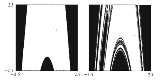
Figure 5: The attraction bassin of the Henon map, β = -0.3 [65].

On the one hand, the black zones in the Figure 5 represent the initial values whose trajectories diverge towards infinity. On the other hand, the white zones represent the initial values that are pulled by the 2-periods attractor. The basin limit is a curve that moves from the inside to the outside of initial values’ space.

The Bernoulli map

This chaotic function is defined in [31] as follows:

      x[n] = y[n-1],

      y[n] = mod(δ.x[n-1], 1)

Where δ is a control parameter set to 1.99 so the map can operate in a chaotic mode [64]. x and y represent the input and the output of the system respectively.

The Mira maps group

The original Mira map  is defined as follows [61]:

x_[n] = y_[n-l],

y_[n] = y_[n-l] – ax_{[n -1]} if  x_{[n -1]} < 6 ,

y_[n] = y_[n-l] + bx_{[n -1]} – 6 (a + b), otherwise

where x and y represent the initial conditions for the trajectory of the map. After numerous trials on the values of the control parameters of the Mira map, we set them during the final experimentation to: a=1.05; and b=2. The modified Mira map is used to imitate the spiking phenomenon of the biological neurons [32], this map is defined as follows:

f(x) = y,

f(y) = a x + b x² + y²

We use this map with the following control parameters’ values:

• Mira_map1, a = 0.8, b = 1, where the map has one breast cancer fixed-point with two positive eigenvalues.
• Mira_map2, a = -0.8, b = 0.2, where the map has a stable set.

The dynamic characteristics of the Mira map and its versions are detailed in [47, 48].

The Spiking maps group

The original Spiking_map is defined in [63] as follows:

Where, x_[n] is the fast dynamical variable, µ is a constant value set at 0.001, y_[n] is the slow dynamical variable, its moderate evolution is on account of to the small value of the parameter µ. The map’s control parameters are the variables α and σ. We use also the Spiking Map with three different modifications. We experiment the parameters’ values used in [63] so that the map operates in a chaotic mode:

• Spiking_Map1: µ = 0.001; α = 5.6 and   σ = 0.322
• Spiking_Map2: µ = 0.001; α = 4.6 and   σ = 0.16
• Spiking_Map3: µ = 0.001; α = 4.6 and   σ = 0.225

      In the present work, we aim at experimenting 23 chaotic maps with the CBAM model, among which we have presented few ones. These selected functions are among the ones that have laid the best accuracy rates.

      Furthermore, we have relied on useful mathematical tools to set the different chaotic maps’ parameters, among which,  the Lyapunov exponent. It represents a logarithmic estimation for the mean expansion rate per cycle of the existing distance between two infinitesimally close trajectories [2]. The interest in the present work concerns particularly the case where that value is positive. It must be noted that, a NDS with a positive Lyapunov exponent characterizes the fact that the system is chaotic. That system is in particular sensible to initial conditions. Figure 6 shows a bifurcation diagram of the Henon map.

For each vertical slice shows the projection onto the x-axis of an attractor for the map for a fixed value of the parameter α.

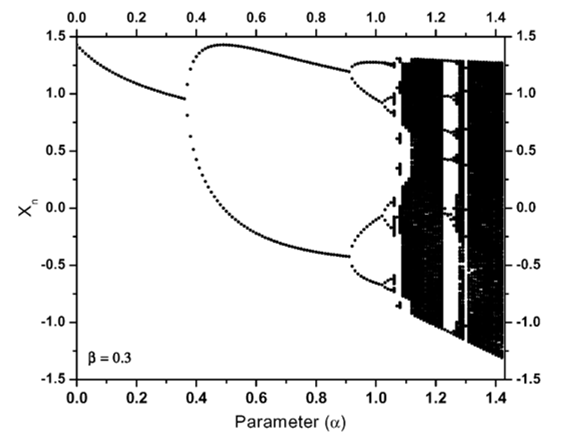
Figure 6: The bifurcation diagram for the Henon map [65].

Whereas, a stable movement has a negative Lyapunov exponent.  An example is illustrated in the Figure 7, which concerns the Henon map Lyapunov Exponent.

Both of those mathematical tools, the bifurcation diagram and the Lyapunov exponent, are useful in our experimental set up to have control over the dynamical behaviors of the performed output unit functions.

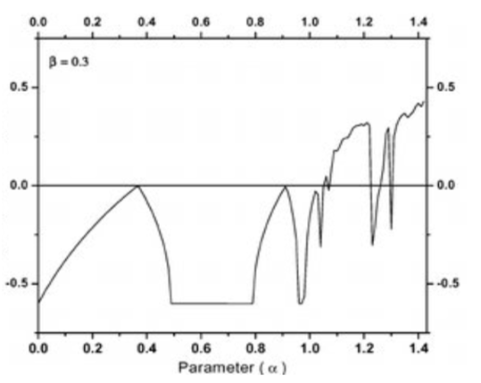
Figure 7: The Lyapunov exponent [65].

3. Data Acquisition

It is a common routine to prepare data before performing the learning and the recall phases on an ANN model. Numerous preprocessing techniques exist in the literature varying according to the nature of the data.  We detail in the following subsections the preprocessing procedure applied on both the set of fluorescence-based measurements, and the breast cancer data collection. It is worth noting here that, noise and missing data are two characteristics that are kept in the datasets.

3.1.  Fluorescence based measurements

A set of fluorescence-based measurements was collected from the optoelectronic biosensor for each analyte at a specific concentration through the procedure detailed in [47]. The first pattern recognition problem to aboard in the present work concerns the identification of different analytes at different concentrations. Table 1 illustrates the test compounds under their different concentrations.

Table 2: Test substances with their concentrations

Compound	Concentration	Category
Chlorophyll	10-4 M 10-5 M 10-6 M 10-7 M 10-8 M	1 2 3 4 5
Coumarin	10-3 M 10-4 M 10-5 M 10-6 M 10-7 M	6 7 8 9 10
Rhomadine B	10-4 M 10-5 M 10-6 M 10-7 M	11 12 13 14
Erythrosin B	10-4 M 10-5 M 10-6 M 10-7 M 10-8 M	15 16 17 18 19

We have 19 classes among which each class represents one compound at a specific concentration.

Concretely, each measurement in the dataset is composed of 64 values forming an 8×8 matrix. The row in the matrix provides the outputs of 7 photodetectors LEDs [47], and one more output corresponding to the excitation LED which is fixed to 0, and then removed leading to the resulting matrix 8×7. Consequently, the size of each vector in the data collection is 56. Furthermore, a random division of the dataset was employed to get two distinct ones, the first one is dedicated to the learning process (two thirds of the entire collection), while the second one is reserved for the testing phase (the remaining third). The resulting datasets contains 2103, and 1051 vectors respectively.

3.2.  Breast Cancer database

      Concerning the second pattern recognition problem investigated in the present work, the authors employ the Yougoslavia Breast Cancer dataset in the experimentations. Clinical data have been collected by Matjaz Zwitter & Milan Soklic at the oncological institute of the university medical center of Ljubljana in Yougoslavia. The entire data collection contain 286 tumor cases. Each tumor case is represented as a vector of 10 attributes: the tumor frequency, the patient age, the type of the menopause, the tumor-size, inv-node, node-caps, deg-malig, breast position, breast-quad, the irradiation value. It must be noted here that few attributes are missing in the breast cancer dataset. The authors apply scaling on the data collection with dividing the values by 10. The digit 0 was excluded to prevent the system from instable fixe points. As a result, the normalized dataset is represented by digits in the interval [1, 13].

Finally, the data collection is composed of  286 tumor cases coded in a set of rows of dimension 10.

Moreover, the different tumor cases  in the breast cancer dataset are not identified. A categorization phase must be accomplished to determine them. As a consequent, the authors developed a Self-Organized Map (SOM), an ANN model detailed in [66]. The designed SOM model consists of a map that is composed of 400 neurons (20*20 cells). Computing units are represented through the matrix cells. As one can notice in Figure 8, the numbers displayed in the 73 cells consist of the resulting categories’ identifiers processed by the SOM network.

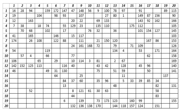
Figure 8: The SOM breast cancers’ categorization

The obtained map indicates that each neuron in the network has the medical specificities of the category that it represents. As a result, the 175 classes (plotted in Figure 8) generated by the SOM are used for breast cancer identification.

For the experimentation needs, and according to the procedure followed in the substance identification task, the breast cancer dataset was separated into two subsets. The first set contains the equivalent of two-thirds (191 vectors), while the second set contains the remaining third (95 vectors). The first dataset is reserved for the training phase, and the second for the recall phase.

The cross-validation method is used to determine the accuracy rates for the different ANN models developed, and this, whether in substance identification task or in the breast cancer detection problem.

4. Experimentations and Results

It is worth noting that, the topology, the activation function and the learning rule are the main parameters that characterizes an ANN model. We detail in the following subsections those parameters in each of the MLNN, the BAM and the C-BAM models.

4.1.  MLNN model

The authors in [47] investigate a set of experimentations on several MLNN architectures and different parameters and converged on the multilayered model employed for the substance identification task. The Stuttgart Neural Networks Simulator (SNNS) of the Stuttgart University in Germany was used for the different MLNN experimentations. The best network performance obtained was with the MLNN topology  consisting of an input layer of the size 56 according to the size of the input vectors, two hidden layers with the same size as the input layer, and one output unit generating the output pattern corresponding to input assigned to the network.  The aforementioned learning algorithm was used as the learning rule, the RProp. The sigmoid was the output function of the MLNN model.

We kept the same conception principle for the breast cancer detection task. The topology of the resulting MLNN model consists of an input layer containing 10 units according to the size of the tumor-case vector, two hidden layers with 10 computing neurons for each, and one output.  The MLNN topology for the breast cancer detection task is plotted in the Figure 9 bellow.

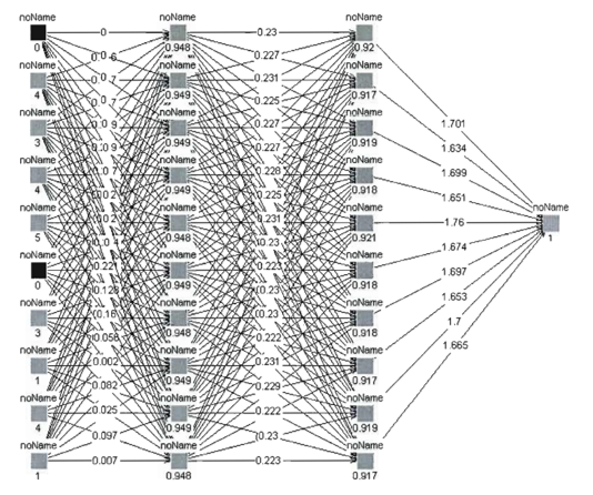
Figure 9: The MLNN topology 10-10-10-1.

The implemented ANN models are tested in the recall phase with the patterns that were not used during the learning process. Meaning that those patterns were not affected to the network during its learning phase, but during the recall only. In addition, the cross validation technique is used to determine the different ANNs’ recognition accuracies. Finally, once the tests are achieved, the average of the three experimentations on each of the ANN models is considered as its overall classification exactitude. Empirically, the MLNN model reached 94,79% of good overall recognition for the substance identification task, 89.32% of exactitude for the breast cancer identification problem.

4.2.  BAM model

The memory-based network architecture is the second ANN model developed in the present work and it is composed of two Hopfield-like neural networks interconnected in head-to-tail fashion, as one can notice in Figure 10. We employ in the BAM model the parameters experimented in [20, 21].

The network topology describes an interconnection that allows a recurrent flow of information that is processed bidirectionally. In that way, the vectors composing the pairs to be learned do not have to be specifically of same dimensions and that, contrary to the conventional BAM designs, the weight matrix from one side is not necessarily the transpose of that from the other side.

The unit activation function employed in the BAM model is the cubic map described in [21]. Figure 4 illustrates the bifurcation diagram of that function according to  the parameter that dictates the dynamic behavior of the outputs.

Fundamentally, this cubic function has three fixed points, -1, 0, and 1, of which both the values-1 and 1 are stable fixed points. They offer to the memory the possibility to develop two attractors at these values. The cubic output function takes several time steps to converge. First, the given stimulus is projected from the network space to the stimuli space. Second, in the following time steps, the stimulus is progressively pushed toward one of the stimuli space corners.

Furthermore, according to Figure 4, one can notice that the learning rule leads to stable attractors for value , when it gets an aperiodic behaviour when exceeding 1 before leading the system into a chaotic phase (black areas in the bifurcation diagram).

The experimentations on the BAM were realized with the cubic map operating in a fixed-points mode. The Hebbian/antiHebbian learning rule includes a feedback from the nonlinear output function via the couple of patterns to be associated; which allows the BAM to learn online, thus contributing to the convergence of the weight connections.

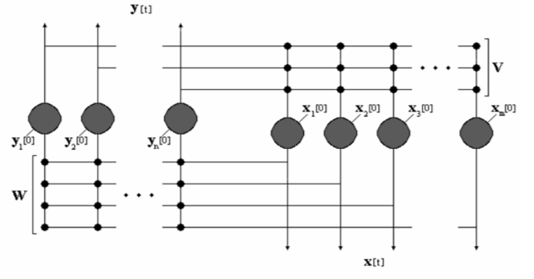
Figure 10: The BAM architecture.

The breast cancer recognition accuracy of the BAM model is plotted in Figure 11.

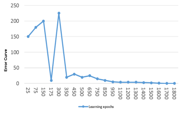
Figure 11: Error curve relative to the number of learning epochs.

The network could reach a steady state after a reasonable number of learning cycles. The error was less than 0,0005 after 1700 epochs. The BAM could correctly categorize 85 tumors cases from the testing dataset. That means that the accuracy rate of the network reached 90,17% at the recall phase. It is worth here that, that recognition rate was accomplished inspite the missing values in the data, which proves a good capacity of generalization on the one hand and a good resilience to noise on the other.

The accuracy increased with the substance identification task to 96,56 % of exactitude. That is certainly due to the better conditions of the data collection despite the larger problem space.

4.3.  CBAM model

The third model developed in the present work is the chaotic BAM model. The same main BAM’s parameters are kept  in the C-BAM network, consisting of the same topology and learning rule as the ones of the former BAM, detailed in [20], except that, the neuron activation function was replaced by chaotic functions. Distinction between the two memory-based ANN models throughout that parameter offers the possibility to concretely estimate the network pattern recognition performance with, and without chaos. The first chaotic output function tested on the C-BAM is the same cubic map employed in the BAM model, operating in a chaotic mode during recall. For that purpose, the value of  was set to 0.1 during training and to 1.5 during recall.As one can notice in Figure 4, those values correspond to a fixed-point and chaotic behavior respectively for that output map. Subsequently, the experimentation of 22 other chaotic maps on the CBAM model were investigated.  Indeed, after reaching a steady state in the learning process, the parameters of each function were fixed so it can operate in a chaotic mode, according to the bifurcation diagram of each map [2, 61, 62, 63, 64].

The recognition accuracy rates are illustrated in Table 2 for both substance identification and the breast cancer identification tasks. For the purpose of results comparison, the MLNN’s and the classical BAM’s performances are also mentioned.

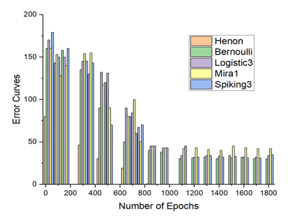
Figure 12: The CBAM error curves for the substance identification’s task with the best 5 performing chaotic maps.

The Figure 12 and the Figure 13 show the best recognition accuracies of the CBAM model with five particular maps, for the substance identification task, and the breast cancer identification task, respectively.

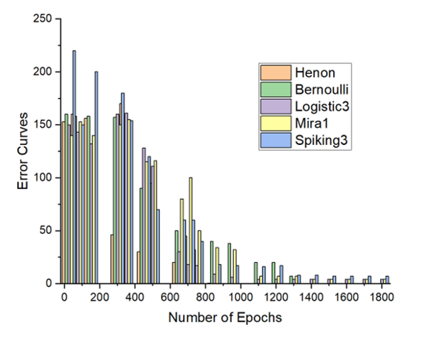
Figure 13: The CBAM error curves for the breast cancers’ recognition task with the best 5 performing chaotic maps.

As one can notice in the above graphs, the accuracy is total in both problem domains, particularly with the Henon function.

5. Conclusion

Three different ANN models were developed in the present work to deal with two different real life problems. Both of those problems focus on pattern recognition, the first task concerns substance identification while the second is about breast cancer detection. On the one hand, the MLNN model reached a good performance at recalling the substance identification data despite the problem of the huge space dimension (56 is the vectors’ size) and the multiclass criterion (19 different classes). The rate was less good for breast cancer identification with the same model in spite of this; the problem of space dimension was diminished to 10. This fact is indicative of the poor generalization capacity of the Multi-Layered Neural Network when data contains noise. In fact, as mentioned in the Data Characteristics section, noise and missing values are two properties that are kept in the datasets. On the other hand, the BAM recurrent model provides a good overall recall for breast cancer identification seeking more that 96% of exactitude. However, the error increased with the multi-class problem relative to fluorescent-based measurements. The BAM results highlight its good resilience to noise; nevertheless, it was less good at facing the large problem space of the fluorescence-based measurements.

In addition, the presence of chaos in the brain-inspired memory-based model provided remarkable results particularly with certain chaotic maps. The recognition accuracy of the CBAM facing the breast cancer detection task was acceptable with six functions employed in a chaotic mode [70% to 89%]; while eight maps varied from good to perfect, reaching a 100% of correct recognition with the Henon and Bernoulli map.  The performance was less good with regard to the substance identification problem compared to the first one, and that is with almost all the chaotic maps except for the Henon map that kept the overall accuracy total. The pattern recognition system employing that particular map was remarkable dealing with both substance identification and breast cancer detection problems. Accordingly, we can state that this particular model encompasses assets which allow it an excellent generalization capacity and a great resilience to noise leading to perfect pattern recognition performance.

 It is crucial to line up future artificial neural networks investigations with the dynamical characteristics of the Henon chaotic function, among which, the fractal dimensions of the Henon attractors. In essence, fractals and modern chaos theory radically question the dynamical concepts in all contexts and more particularly in nature and its mimetic artificial systems, among which, artificial neural networks.  Besides, and to conclude, since it is the era of big data; chaos must imperatively be in the perspectives of deep learning techniques in artificial neural network models’ analytics.

Conflict of Interest

The authors declare no conflict of interest.

Acknowledgment

This study was funded by the Algerian ministry of higher education and scientific research and the General Directorate for Scientific Research and Technological Development (DG-RSDT).

This work was also possible thanks to the financial support of excellence scholarships foundation of the University of Quebec at Montreal (UQAM) for graduate studies, Montreal, Quebec, Canada. Many thanks to the Texas-center of Superconductivity and Advanced Materials (TcSAM) in the Physics Department of the University of Houston, Houston, Texas, USA, for allowing us to use their data in our experimentations.

1. H. Naoum, S. Benslimane, M. Boukadoum, “Classical and Brain-inspired Neural Networks for Substance Identification and Breast Cancer Detection: The Chaos Challenge,” The first international conference on Cyber Management and Engineering (CyMaEn`21), IEEE, 1–6, 2021, doi: 10.1109/CyMaEn50288.2021.9497280.
2. K. T. Alligood, T. D. Sauer, J. A. Yorke, “Chaos: An Introduction to Dynamical Systems,” Textbook in Mathematical Sciences. Springer, New York, NY, 105–147, 1996, doi:10.1007/b97589.
3. W. J Freeman, “Simulation of chaotic EEG patterns with dynamic model of the olfactory system,” Biological Cybernetics, 56(2–3), 139–150, 1987.
4. H. Korn, P. Faure, “I there chaos in the brain? Experimental evidence and related models,” Neurosciences, 326(9), 787–840, 2003.
5. A. Combs, S. Krippner. W. Freeman, “III and the chaotic nature of deams,” Nonlinear Dynamics, Psychology and life sciences, 21(4), 475-484, 2017.
6. V. V. Kozlova, V. A. Galkin, M. A. Filatov, “Diagnostics of brain neural network states from the perspective of chaos,” Journal of physics: conference series. 1889 052016, 2021, doi:10.1088/1742-6596/1889/5/052016.
7. M. AR. Thabet, “Quantum chaos and the brain,” IBCHN – Imperial Collage – Michael Crawford’s Lab, 2020, doi:10.13140/RG.2.2.20160.48645.
8. B. Yan, S. Mukherjee, A. Saha, “Exploring noise-induced chaos and complexity in a red blood cell system,” Springer, The European Physical Journal Special Topics, 230, 1517–1523, April 2021, doi:10.1140/epjs/s11734-021-00030-2.
9. N. B. Harikrishnan, N. Nagaraj, “When noise meets chaos: stochastic resonanace in neurochaos learning,” Elseivier, 143, 425–435. Special Issue, 2021, doi:10.1016/j.neunet.2021.06.025.
10. G. Eason, B. Noble, I. N. Sneddon, “On certain integrals of Lipschitz-Hankel type involving products of Bessel functions,” Phil. Trans. Roy. Soc. London, A247, 529–551, April 1955, doi:10.1098/rsta.1955.0005.
11. A. Babloyantz, C. Lourenc-o, “Computation with chaos: A paradigm for cortical activity,” Proceedings of the National Academy of Sciences, 91, 9027–9031, 1994, doi:10.1073/pnas.91.19.9027.
12. M. P. Dafilis, D. T. J. Liley, P. J. Cadusch, “Robust chaos in a model of the electroencephalogram: Implications for brain dynamics,” Chaos, 11, 474–478, 2001, doi:10.1063/1.1394193.
13. H. Korn, P. Faure, “Is there chaos in the brain? II. Experimental evidence and related models,” Comptes Rendus Biologies, 326(9), 787–840, 2003, doi:10.1016/j.crvi.2003.09.011.
14. M. A Rozhnova, E. V Pankratova, S. V Stasenko, V. B Kazantsev, “Bifurcation analysis of multistability and oscillation emergence in a model of brain extracellular matrix,” Elseivier, Chaos, Solitons & Fractals, 151, October 2021, doi:10.1016/j.chaos.2021.111253.
15. A. Wu, Y. Chen, Z. Zeng, “Quantization synchronization of chaotic neural networks with time delay under event-triggered strategy,” Springer Verlag, Cognitive Neurodynamics, 15, 897–914, 2021, doi: 10.1007/s11571-021-09667-0.
16. M. Negnevitsky, “Artificial Intelligence: A guide to Intelligent Systems,” Addison Wesley, 3rd edition, 2011.
17. K. Saravanan, S. Sasithra, “A review on Classification Based on Artificial Neural Networks,” International Journal of Ambient Systems and Applications (IJASA), 2(4), 11–18, 2014, doi:10.5121/ijasa.2014.2402.
18. S. Haykin, “Neural networks: A comprehensive foundation,” Englewood Cliffs, NJ: Prentice-Hall, 1999.
19. T. Kohonen, “Correlation matrix memories,” IEEE Trans. Comput. , C-21, 353–359, Dec. 1972, doi: 10.1109/TC.1972.5008975.
20. S. Chartier, M. Boukadoum, “A bidirectional Heteroassociative Memory for binary and Grey-Level Patterns, “ IEEE Transactions on Neural Networks, 17(2), March 2006, doi: 10.1109/TNN.2005.863420.
21. S. Chartier, M. Boukadoum, “Encoding static and temporal patterns with a bidirectional heteroassociative memory,”Journal of applied mathematics, 20011, 1–34, 2011, doi: 10.1155/2011/301204.
22. S. Chartier, S. Helie, M. Boukadoum, R. Proulx, “SCRAM: statistically converging recurrent associative memory,” IEEE International Joint Conference on Neural Networks, IJCNN, 2005, doi: 10.1109/IJCNN.2005.1555941.
23. S. Chartier, M. Renaud, M. Boukadoum, “A nonlinear dynamic artificial neural network model of memory,” New Ideas in Psychology, 26(2), 252–277, 2008, doi:10.1016/j.newideapsych.2007.07.005.
24. M. Adachi, K. Aihara, “Associative dynamics in a chaotic neural network. Neural Networks,” 10(1), 83–98, 1997, doi:10.1016/S0893-6080(96)00061-5.
25. K. Aihara, T. Takabe, M. Toyoda, “Chaotic neural networks,” Physics Letters A, 144(6–7), 333–340, 1990, doi:10.1016/0375-9601(90)90136-C.
26. H. Imai, Y. Osana, M. Hagiwara, “Chaotic analog associative memory,” Systems and Computers in Japan, 36(4), 82–90, 2005, doi: 10.1109/IJCNN.2001.939522.
27. R. S. T. Lee, “e-associator: A chaotic auto-associative network for progressive memory recalling,” Neural Networks, 19(5), 644–666, 2006, doi: 10.1016/j.neunet.2005.08.017.
28. Y. Osana, M. Hagiwara, “Knowledge processing system using improved chaotic associative memory,” Proceeding of the International Joint Conference on Neural Networks (IJCNN’00), 5, 579–584, 2000.
29. U. Ozdilek, “Value order in disorder,” Springer, International Journal of Dynamics and Control, 2022, doi:10.1007/s40435-021-00903-3.
30. H. Lin, C. Wang, Q. Deng, C. Xu, Z. Deng, C. Zhou, “Review on chaotic dynamics of memristive neuron and neural network,” Nonlinear Dynamics, 106, 959–973, 2021, doi:10.1007/s11071-021-06853-x
31. Y. Zhang, Y. He, F. Long, “Augmented two-side-looped Lyapunov functional for sampled-data-based synchronization of chaotic neural networks with actuator saturation,” Elsevier, Journal of Neurocomputing, 422, 287–294, 2021, doi:10.1016/j.neucom.2020.09.018.
32. C. Chen, A. Abbott, D. Stilwell, “Multi-Level generative chaotic recurrent network for image inpainting,” Proceedings of the IEEE CVF winter conference on applications of computer vision (WACV), 3626-3635, 2021, doi: 10.1109/WACV48630.2021.00367.
33. H. Kaur, A. Bhosale, S. Shrivastav, “Biosensors: Classification, fundamental characterization and new trends: A Review,” International Journal Of Health Sciences and Research, 8(6), 315–333, 2018.
34. M. H. Mozaffari, L. Tay, “A review of 1D Convolutional Neural Networks toward Unknown Substance Identification in Portable Raman Spectrometer,” arXiv:2006.10575 [eess.SP] (2020).
35. R. Fleh, M. Othman, S. Gomri, “WO3 sensors array coupled with pattern recognition method for gases identification,” 13th International Multi-Conference on systems, Signals and Devices, IEEE, 147–152, 2016.
36. D. Karakaya, O. Ulucan, M. Turkan, “Electronic nose and its applications: A survey,” International Journal of Automation and Computing, 17, 179–209, 2020, doi:10.1007/s11633-019-1212-9.
37. B. Podola, M. Melkonian, “Genetic programming as a tool for identification of analyte-specificity from complex response patterns using a non-specific whole-cell biosensor,” Biosensors and Bioelectronics 33, 254-259, 2012, doi: 10.1016/j.bios.2012.01.015.
38. M. Kukade, T. Karve, D. Gharpure, “Identification and classification of spices by Machine Learning,” IEEE International Conference on Intelligent Systems and Green Tchnology (ICISGT), 2019, doi: 10.1109/ICISGT44072.2019.00015.
39. A. L. Vazquez, M. M. Domenech Rodriguez, T. S. Barrett, S. Schwartz, N. G. Amador Buenabad, M. N. Bustos Gamino, M. L. Gutierrez Lopez, J. A. Villatoro Velazquez, “Innovative Identification of Substance Use Predictors: Machine Learning in a National Sample of Mexican Children,” Journal of Society for Prevention Research, Springer-Verlag, 2020, doi: 10.1007/s11121-020-01089-4.
40. F. L. Melquiades, A. Mattos Alves da Silva, “Identification of sulphur in nail polish by pattern recognition methods combined with portable energy dispersive X-ray fluorescence spectral data,” Journal of Analytical Methods, 8, 3920–3926, 2016, doi:10.1039/C6AY00195E.
41. Z. Almheiri, M. Meguid, T. Zayed, “Intelligent Approaches for predicting failure of water mains,” Journal of Pipeline Systems Engineering and Practice, 11(4), 1949–1190, 2020, doi:10.1061/(ASCE)PS.1949-1204.0000485.
42. F. Hu, M. Zhou, P. Yan, K. Bian, R. Dai, “PCANet: A common solution for laser-induced fluorescence spectral classification,” IEEE Access 7, 2169–3536, 2019, doi: 10.1109/ACCESS.2019.2933453.
43. L. G. Zhang, X. Zhang, L. J. Ni, Z. B. Xue, X. Gu, S X. Huang, “Rapid identification of adulterated cow milk by non-linear pattern recognition methods based on near infrared spectroscopy,” Food Chemistry 145, 342–348, 2014, doi:10.1016/j.foodchem.2013.08.064.
44. P. T. Hernandez, S. Hailes, I. P. Parkin, “Cocaine by-product detection with metal oxide semiconductor sensor arrays,” Royal Society of Chemistry, 10, 28464–28477, 2020, doi:10.1039/D0RA03687K.
45. Y. Hui, X. Xue, Z. Xuesong, W. Yan, Z. Junjun, “Bacteria strain identification with fluorescence spectra,” Applied Mechanics and Materials, 865, 630–635, 2017, doi:10.4028/www.scientific.net/AMM.865.630.
46. L. Poryvkina, V. Aleksejev, S. M. Babichenko, T. Ivkina, “Spectral pattern recognition of controlled substances in street samples using artificial neural network system,” Optical Pattern Recognition, Proceedings of SPIE, 8055, 2011, doi:10.1117/12.883408.
47. H. Naoum, M. Boukadoum, C. Joseph, D. Starikov, A. Bensaoula, “Intelligent Classifier Module for Fluorescence Based Measurements,” Proc. International Workshop on Signal Processing and its Applications (WoSPA 2008), Sharjah (UAE), 18–20 2008.
48. N. Nouaouria, M. Boukadoum, “A Particle Swarm Optimization Approach for Substance Identification,” The Genetic and Evolutionary Computation Conference (GECCO), 1753–1754, 2009, doi:10.1145/1569901.1570142.
49. A. R. Vaka, B. Soni, R. K. Sudheer, “Breast Cancer Detection by leveraging Machine Learning,” The Korean Institute of Communication and Information Sciences (KICS), 10–1016, 2020, doi:10.1016/j.icte.2020.04.009.
50. H. Jouni, M. Issa, A. Harb, G. Jacquemod, Y. Leduc, “Neural Network Architecture for Breast Cancer Detection and Classification,” IEEE International Multidisciplinary Conference on Engineering Tchnology (IMCET), 987-1-5090-5281-3, 2016, doi: 10.1109/IMCET.2016.7777423.
51. S. Sharma, A. Aggarwal, T. Choudhury, “Breast Cancer Detection Using Machine Learning Algorithms,” International conferfence on computational techniques, electronics and mechanical systems (CTEMS), IEEE, 2019, doi: 10.1109/CTEMS.2018.8769187.
52. J. Sivapriya, V. Aravind Kumar, S. Siddarth Sai, S. Sriram, “Breast cancer prediction using machine learning,” International Journal of Recent Technology and Engineering (IJRTE), 8(4), 2019, doi:10.35940/ijrte.D8292.118419.
53. K. Santhosh, T. Daniya, J. Ajayan, “Breast Cancer Prediction Using Machine Learning Algorithms,” International Journal of Advanced Science and Technology, 29(3), 7819–7828, 2020.
54. B. Karthikeyan, G. Sujith, H. V. Singamsetty, P. V. Gade, S. Mekala, “Breast cancer cetection using machine learning,” International Journal of Advanced Trends in Computer Science and Engineering, 9(2), 981–984, 2020, doi:10.30534/ijatcse/2020/12922020.
55. A. E. Bayrak, P. Kirci, T. Ensari, “Comparison of machine learning methods for breast cancer diagnosis,” Scientific Meeting on Electrical-Electronics and Biomedical Engineering and Computer Science (EBBT), Istambul, Turkey, 1-3, 2019, doi: 10.1109/EBBT.2019.8741990.
56. M. Karabatak, “ New classifier for breast cancer detection based on Naïve Bayesian,” Measurement. 72, 32–36, 2015.
57. B. Li, C. Delpha, D. Diallo, A. Migan-Dubois, “Application of artificial neural networks to photovoltaic fault detection and diagnosis: A review,” Elsevier, Renewable and Sustainable Energy Reviews, 138, 2021, doi:10.1016/j.rser.2020.110512.
58. M. Riedmiller, H. Braun, “A direct adaptive method for faster backpropagation learning: the RPROP algorithm,”IEEE International Conference on Neural Networks, 1993, doi: 10.1109/ICNN.1993.298623.
59. J. Han, C. Moraga, “The influence of the sigmoid function parameters on the speed of backpropagation learning,” Springer Verlag, International Workshop on Artificial Neural Networks, 195–201, 1995, doi:10.1007/3-540-59497-3_175.
60. B. Kosko, “Bidirectional associative memories,” IEEE Trans. Syst., Man, Cybern., 18(1), 49–60, Jan.-Feb, 1988, doi: 10.1109/21.87054.
61. I. Gumowski, C. Mira, “Recurrences and discrete dynamic systems,” Lecture notes in mathematics, book series, 809, 1980, doi:10.1007/BFb0089135.
62. J. P. England, B. Krauskopf, H. M. Osinga, “Computing One-Dimensional Stable Manifolds and Stable Sets of Planar Maps without the Inverse,” SIAM J. Applied Dynamical Systems, Society for Industrial and Applied Mathematics, 3, 161–190, 2004, doi:10.1137/030600131.
63. A. L. Shilnikov, N. F. Rulkov, “Origin of Chaos in a Two-Dimensional Map Modeling Spiking-Bursting Neural Activity,” International Journal of Bifurcation and Chaos (IJBC), 13(11), 3325–3340, 2003, doi:10.1142/S0218127403008521.
64. S. J. Baek, E. Ott, “Onset of synchronization in systems of global1y coupled chaotic maps,” Physical Review Letters, 69(6), 066210 2004, doi: 10.1103/PhysRevE.69.066210.
65. V. Patidar, G. Purohit, K.K Sud, “Dynamical behavior of q-deformed Hénon map”. International journal of bifurcation and chaos, 21(05), 1349–1356, 2011, doi:10.1142/S0218127411029215.
66. T. Kohonen, “Self-Organizing Maps,” In: Sammut C., Webb G.I. (eds) Encyclopedia of Machine Learning. Springer, 2011, doi:10.1007/978-0-387-30164-8_746.

(Click Here)