1. Introduction

Lung cancer is the leading cause of cancer-related deaths (18.0% of the total cancer deaths), followed by colorectal (9.4%), liver (8.3%), stomach (7.7%), and female breast (6.9%) cancers [1]. Early diagnosis and treatment may save lives. Although computerized tomography (CT) scan imaging is the best imaging technique in the medical field, it is difficult for doctors to interpret and identify cancer using CT scan images [2]. In addition, because lung cancer detection can increase the detection time and error rate depending on the skill of the doctor, computer-aided diagnosis (CAD) studies to passively assist the detection are on image segmentation, denoising, and 3D image processing using image processing [3] and neural network optimization [4–6].

To improve the anatomical interpretation ability of CT images, this study is designed to improve the cognitive ability of detectors by setting lung, soft tissue, and bone as the regions of interest and utilizing a dataset which is visually easy to distinguish between each region’s features in deep learning.

In the dataset construction phase, the dataset was constructed by preprocessing the Digital Imaging and Communications in Medicine (DICOM) files provided by the Lung-PET-CT-Dx dataset [7,8]. The region of interest to which Hounsfield Unit (HU) windowing is applied is composed of a fundamental three-channel dataset (3ch-ORI) to generate an image, and the characteristics of each region can be recognized in one image. Because this process can improve the cognitive ability to visually classify the regions of interest, it is relevant to feature extraction through anatomical analysis in the training process of a neural network, mimicking the human brain and lung cancer detection process. In addition, to enhance the contrast of the 3ch-ORI, a detector with optimal performance was selected by comparing the results of deep learning on a dataset (3ch-CLAHE) to that which the contrast-limited adaptive histogram equalization (CLAHE) was applied. Considering the deep learning phase, deep learning was performed using reference datasets and a reference detector to determine the optimal train customization settings.

The Lung-PET-CT-Dx dataset used in this study provides version 1 (release date: June 1, 2020) to version 5 datasets (release date: December 22, 2020); nonetheless, it has been released recently and the related studies [9,10] are insufficient. Therefore, in the evaluation stage, the raw original dataset (1ch-ORI) was used as a reference for comparison. Regarding performance evaluation, the intersection of union (IoU) was calculated to achieve high-level results with a sensitivity, precision, and F1-score rates of 94.90%, 96.70%, and 95.56%, respectively.

2. Related studies

This chapter describes the existing studies that have used methods such as structural separation, noise removal, and three-dimensional (3D) technology for visualization of CT images using the Lung Image Database Consortium and Image Database Resource Initiative dataset (LIDC-IDRI). A novel objective evaluation framework for nodule detection algorithms using the largest publicly available LIDC-IDRI dataset or subset lung nodule analysis 2016 (LUNA16) is a challenge [11]. This set of additional nodules for further development of the IDRI-IDRI dataset that was initiated by the National Cancer Institute (NCI) [12,13] have been released.

In [14], they proposed a novel pulmonary nodule detection CAD system and developed to detect nodule candidates using improved Faster R-CNN. They have archived sensitivity of 94.6%. In [15], the noise present in the CT image was removed by applying the weighted mean histogram equalization (WMHE) method, and the quality of the image was improved using the improved profit clustering technique. Consequently, minimum classification errors of 0.038% and 98.42% accuracies were obtained. The method [16] using the modified gravity search algorithm (MGSA) for the classification and identification of lung cancer in CT images achieved a sensitivity, specificity, and accuracy of 96.2%, 94.2%, and 94.56%, respectively, owing to the application of the optimal deep neural network (ODNN). Furthermore, a threshold-based technique for separating the nodules of lung CT images from other structures (e.g., bronchioles and blood vessels) was proposed [17], and from the evaluation, a sensitivity of 93.75% was achieved. The 3D region segmentation of the nodule in each lung CT image achieved 83.98% [18] because of image reconstruction using the sparse field method. In many other studies, many methods for detection and classification using image processing and deep learning have been proposed, and their performance is quite high. These studies aimed at assisting medical staff with visualization based on image processing. Therefore, various methods need to be continuously studied for CAD systems, where even a 0.01% performance improvement is significant. In this study, the improved CT image is used for deep learning to improve the anatomical analysis ability of each region of interest in the CT image. The dataset aimed at enhancing the quality of the CT image in the pre-processing of the DICOM file without using a complicated image processing method to achieve a high level of result. If the improved CT image is applied to the method proposed in previous studies, a better performance is expected.

3. Materials and Methods

3.1.  Dataset construction phase

The preprocessing step of this study includes obtaining a purified CT image through structural analysis of the Lung-PET-CT-Dx dataset, pixel range normalization of the DICOM file, and HU windowing for each region of interest. The Lung-PET-CT-Dx dataset consists of CT and PET-CT DICOM images of lung cancer subjects with XML annotation files that indicate tumor location with bounding boxes.  The subjects were grouped according to tissue histopathological diagnosis. Patients with names/IDs containing letter ‘A’ were diagnosed with Adenocarcinoma, ‘B’ corresponded to Small Cell Carcinoma, ‘E’ indicated Large Cell Carcinoma, and ‘G’ corresponded to Squamous Cell Carcinoma [19].

Object detection performs classification and localization to obtain detection and classification results for each class. However, because this study focuses on the performance of detecting lung cancer, one class was evaluated using only the adenocarcinoma class, without using a dataset with a different number for each class. Therefore, the results of the classification are meaningless, and only the results of localization are used to evaluate the performance. The adenocarcinoma class consists of sub-directories divided for each slice in 265 main directories, and 21 main directories that do not have annotation files or do not match the annotation xml information are excluded from the dataset configuration. In addition, the DICOM files existing in each directory were merged into one directory for easy management and quick data access. The annotation files matching 1:1 with the DICOM file were stored in one common csv file, and after xml parsing, they were stored in the DICOM file. Unlike greyscale images which are in a range of 0 to 255, DICOM files are converted to 12-bit pixel arrays, and DICOM files are composed of HU [20] (a unit that expresses the degree of attenuation of X-rays when penetrating the body). Therefore, as shown in Figure 1, the DICOM file can be viewed more clearly by normalization and HU windowing.

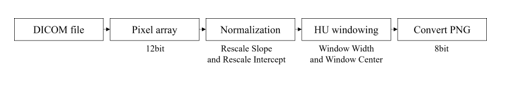
Figure 1: Process steps of the DICOM file

First, the 12-bit (4096 level) pixel array extracted from the DICOM image was normalized according to the unit defined in the HU. Depending on the CT equipment, the pixel range was stored as 0 to 4095 or -2048 to 2047. Using Equation (1), linear transformation was applied to the ‘Rescale slope’ and ‘Rescale intercept’ fields to remap the image pixel:

    Out pixel = rescale slope * input pixel + rescale intercept (1)

For example, as shown in the figure, in the 0-to-4095-pixel range, the rescale intercept has a value of − -2048, and the rescale slope has a value of 1; therefore Equation (1) is used to convert it to a value in the range of − -2048 to 2047. In contrast, the rescale intercept of the DICOM file stored in the pixel range of -2048 to 2047 is 0; hence, there is no change even if the above formula is used. Therefore, normalization is applied to the range shown in Figure 2, and all DICOM files are placed within the same pixel range. Considering the reference, dataset, the rescale slope and rescale intercept attributes do not exist in the properties of the DICOM file, they are excluded from the dataset configuration.

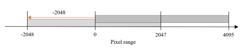
Figure 2: Brightness settings for DICOM image

Subsequently, the normalized pixel array performs the HU windowing process by applying the window width and center properties to each region of interest as shown in Table 1.

Table 1: Window setting using the Hounsfield Unit

Window	Lung	Soft tissue	Bone
Window Center	-700	40	500
Window Width	1400	350	2000

The overall flow of the data construction phase that processes the DICOM file and composes each dataset is shown in Figure 3.

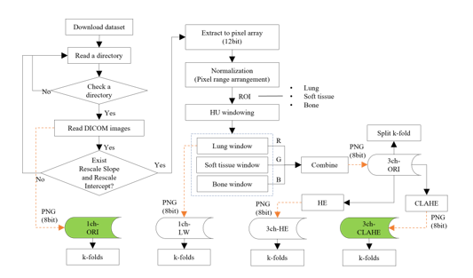
Figure 3: Flow of the dataset construction phase

In dataset composition step, a method of composing an image in three-channel and generating images with enhanced contrast by applying CLAHE is described. The CLAHE is an algorithm that uniformly divides an image and distributes pixels of a specific height to each area. After setting the clip limit (the threshold), the height of the histogram was limited.

Table 2 lists the composition and use of the dataset employed. The 1ch-ORI is a dataset consisting of images converted directly into a PNG format from the original DICOM image without any processing and is used as a reference in the experiment. On the contrary, the 3ch-HE, which applies histogram equalization (HE) equally to all pixels, is used as a reference dataset for comparison with the 3ch-CLAHE. In addition, the 3ch-ORI is a fundamental three-channel dataset before the application of equalization.

Table 2: Datasets used for the experiment

Name	Configuration	Usage
1ch-ORI	Raw dataset	Reference dataset
3ch-ORI	3-channel dataset before equalization	Fundamental dataset of 3-channel
3ch-CLAHE	3-channel dataset after CALHE	Proposed dataset
3ch-HE	3-channel dataset after HE	Reference dataset for equalization

Contrast enhancement using image processing can acquire more detailed information by improving visual recognition ability; thereby, increasing the analysis ability of CT images in the process of human visual and feature recognitions in deep learning. Because methods such as linear combination [21] used for contrast enhancement use multiple images for one-channel, it may affect the contrast range when observing the HU-applied window. Contrast enhancement is a specific characteristic enhancement of image enhancement processing. Histogram equalization is a popular method for image contrast enhancement [22]. Therefore, in this study, the histogram processing technique is applied to the 3ch-ORI, in which the window of interest is set as the data for each channel. However, histogram equalization is not the best method for contrast enhancement because the mean brightness of the output image is significantly different from that of the input image [23]. Brightness is used as an important feature along with shape information when configuring channels, and it is difficult to distinguish between regions because CT images that are not pre-processed may be dark and noise may exist as shown in Figure 4-(A). The histogram can be divided into left, right, and midtones. In Figure 4-(B), where equalization is not applied, the highlighted area is empty; hence, it is difficult to distinguish each area as dark as shown in Figure 4-(A).

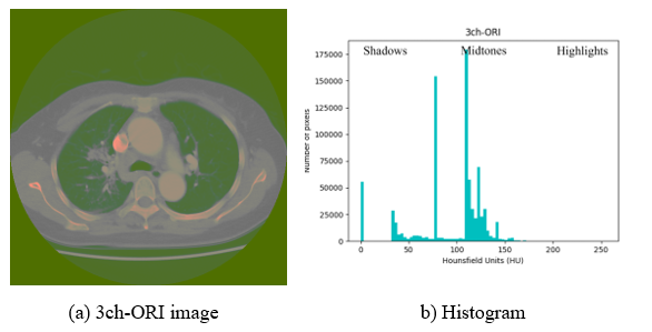
Figure 4: Exemplary image and histogram of 3ch-ORI

If HE is applied to all pixels at once, equalization is performed indiscriminately. This may cause noise in extremely dark or bright areas or loss of necessary information. Considering Figure 5-(B), where histogram equalization is applied, the number of pixels in the highlighted area is increased (yellow dotted arrows), and it can be seen that Figure 5-(A) affects the increase in pixel intensity and brightness. However, the midtone area decreased, resulting in the spread of shadow and highlight directions. Because it is more difficult to classify each area owing to the addition or loss of information in a specific area, the CLAHE method is used in this study to prevent noise overamplification.

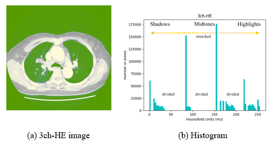
Figure 5: Example image and histogram of 3ch-HE

In Figure 6, to which CLAHE is applied, it can be observed that the level of pixel areas is spread around the midtone area (yellow dotted arrows), the number of pixels is evenly distributed, and the average value is decreased (orange dotted arrows), enhancing the contrast.

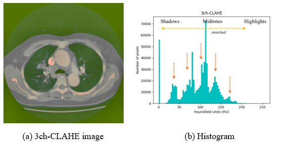
Figure 6: Exemplary image and histogram of the 3ch-CLAHE

In Figure 4, the contrast is too low to distinguish each region using human eyes; therefore, Figures 5 and 6 with enhanced contrast are used for the experiment. Considering a human point of view, the characteristics of each area in Figure 6 can be distinguished better than in Figure 5; nevertheless, an accurate judgment is made by comparing the deep learning results. Equalization of the histogram using brightness rather than the color of the image was applied after configuration as three three-channels because if three three-channels were configured by applying them to each gray image, different contrasts could be applied to each channel. Therefore, because it is different from the intended image when combined with the color model, three-channel, unintended results of anatomical organs, structures, or artifacts in the human body can have a significant impact on CT image analysis.

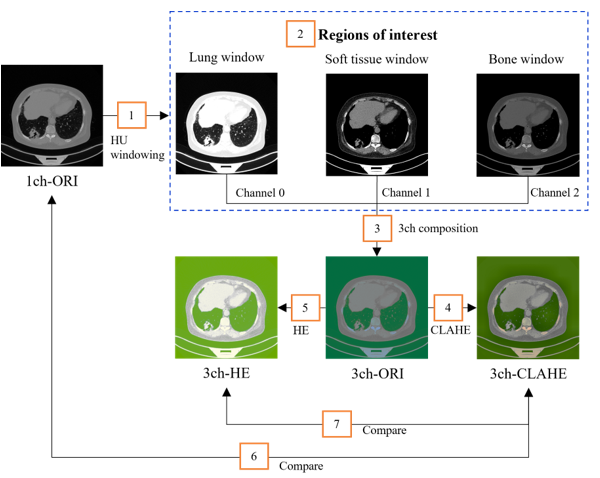
Figure 7:  Dataset construction flow

The configuration flow of the dataset is shown in Figure7. The three types of areas of interest (number 2 in the orange box), lung, soft tissue, and bone window, appear clearly after HU windowing. However, it is difficult to anatomically distinguish each area owing to the addition or loss of the specific areas.

After applying each method in the 12-bit pixel array, each dataset was converted to an 8-bit PNG format and stored on a disk. A total of 13,233 images were divided into train- and test-sets in a ratio of 8:2 (10,586:2,647). In addition, because data bias in each dataset can affect the evaluation results of the deep learning model, five-fold cross-validation was performed as shown in Figure 8 to select the optimal fold to be used in the experiment.

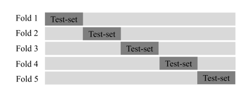
Figure 8:  Dataset composition of the cross-validation

3.2.  Deep Learning phase

In general, object detection is categorized into one- and two-stage detectors as shown in Table 3. One-stage detectors perform classification and localization concurrently. Therefore, they are fast; however, they are low in accuracy. The two-stage detectors use the Legion Proposal Network (RPN) to select candidate areas where objects are expected to be detected, making them slow; nonetheless, they are high in accuracy. The most recent one-stage detectors exceed the accuracy of two-stage detectors; hence, classification according to accuracy is less meaningful.

In this study, we compared RetinaNet [24] using two-dimensional (2D) image-based anchor-based detectors and Faster R-CNN [25–27]  as a reference, modified and utilized Faster R-CNN [28,29] and RetinaNet [30] cloned from the GitHub repository to create a model.

Table 3: Comparison of one- and two-stage detectors

Detector	Anchor based	Detector (Deep learning algorithm)
one-stage	O	YOLO-v1, v2, v3 (2016), SSD (2016) – RetinaNet (2017)
	X	CornerNet (2018) – ExtremeNet (2019) – CenterNet (2019)
two-stage	O	R-CNN (2013) – Fast R-CNN (2015) – Faster R-CNN (2015) – Mask RCNN (2017)

In deep learning, train customization is an important experimental step for selecting the optimal dataset configuration and detector. In this study, ResNet-{50, 101, 152} pretrained with ImageNet [31] was used for transfer learning, and random flip and data shuffle were applied for data augmentation. Moreover, for stable optimization, Adam [32] was used as the optimizer, and the learning rate was set to 1e-5. Considering the reference, Faster R-CNN, which is divided into two stages of RPN and classifier, sets the customization of both elements similarly. Furthermore, the epoch size was set to 500, and the batch size was set to four or eight. Experiments were performed in the environment of Python 3.7, Cuda-10, and a GPU on a 64bit Ubuntu18.04LTS operating system.

After generating a model using the training set and evaluating it using the test set, the overall flow of the deep learning phase (the process of determining the final performance) is shown in Figure 9.

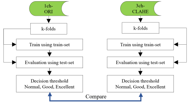
Figure 9:  Flows of the deep learning phase

Object detection performs both classification, which classifies objects in the bounding box, and localization, which is a regression process for finding the bounding box. However, because the classification performance of this study is recognized as only one class using a single class, it is not reflected in the evaluation, and the IoU of the bounding box detected by localization and the ground truth (GT) box, which is the annotation information, is calculated. Considering the reference dataset, when multiple bounding boxes are detected in the test-set image, the bounding box with the highest IoU is selected as the IoU of the image. In many cases, natural scene images can be judged by predicting low-level detection results of objects such as people or automobiles with the human eye. However, lung cancer tumors have a non-standard shape; thereby, requiring a higher performance. In this study, to increase the reliability of the detection performance as shown in Table 4, the decision thresholds for each image are set to be narrower than those of the natural scene image for final judgment. However, the narrower the threshold setting range is, the higher the reliability and the lower the statistical evaluation results. Because the achievement result can be relatively decreased, it must be carefully set according to the field of use

Table 4: Setting of the decision threshold

Decision	Natural scene	Proposed
Normal	>=0.50	>=0.60
Good	>=0.70	>=0.75
Excellent	>=0.90	>=0.90

Table 5: Confusion matrix

Name	Threshold	Description
TP	>= 0.6	Lung cancer exists, detected correctly
TN	No use	No lung cancer exists, identified correctly
FP	< 0.6	No lung cancer exists, detected incorrectly
FN	–	Lung cancer exists, missed

The evaluation of models using the test-set images uses the outcomes of four kinds of statistical confusion matrices as shown in Table 5. True Positive (TP) is determined to correctly detect lung cancer tumors when the IoU is 0.6 or higher, and false positive (FP) is determined to be incorrectly detected when the IoU value of the detected bounding box is 0.6 or less. Considering the false negatives (FN), because there is no detected bounding box, the IoU for the GT box cannot be calculated; therefore, a value excluding TP from the total dataset is used. Regarding the reference dataset, negative (TN) is used when lung cancer tumors do not exist and is not used in the field of object detection for a dataset consisting of one class in which the GT box exists in all the test-set images. The total test-set image length and number of GT boxes were the same.

The experimental results were evaluated using statistical performance measurement methods such as sensitivity, precision, and F1-score. Sensitivity represents the predicted positive among all positives and is calculated using Equation 2:

                    Sensitivity (or Recall) = TP / (TP + FN)               (2)

Precision is the proportion of true positives among the predicted positives, calculated using Equation 3:

                               Precision = TP / (TP + FP)                          (3)

Because the indicators of sensitivity and precision are inversely proportional, it cannot be concluded that a high value of one of them has good performance. Finally, the F1-score is a harmonic mean that considers both sensitivity and precision. The optimal value is one, and the higher the value is, the better the performance, and it is calculated using Equation 4:

F1-score = 2 * (Precision * Recall) / (Precision + Recall)  (4)

3.3.  Results and Discussion

In this chapter, experiments are conducted using each evaluation element, as shown in Figure 10, and the results are discussed.

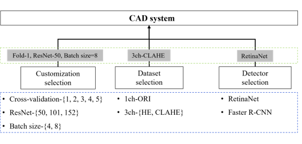
Figure 10:  Evaluation factors and flows.

Train customization selection (blue dotted box) through cross-validation experiments, ResNet-depth, and batch size. The data selection and detector selection steps describe the process of selecting a detector with the best performance (green dotted box) through evaluation and using it as a CAD system. First, the experimental results of train customization according to the conditions of cross validation, ResNet-depth, and batch size for the selection of a detector to be used in the CAD system are shown in Table 6. When the Fold-Num was set to one and the batch size was set to eight, the highest result was a sensitivity of 94.9% and precision of 96.7% in ResNet-50, and the F1-score result was the highest in ResNet-101 with 95.8%. Considering the reference dataset, the result of the F1-score in ResNet-50 was 95.6%, being the second highest result.

Table 6: Comparison of ResNet-50 that changed the conditions of customization and ResNet-{101, 152}

Fold	Depth	Batch Size	Sensitivity (%)			Precision (%)			F1-score (%)
			Normal	Good	Excellent	Normal	Good	Excellent	Normal	Good	Excellent
1	50	8	94.9	72.3	14.5	96.7	73.9	14.8	95.6	73.1	14.6
2	50	8	93.7	72.9	13.8	96.3	75.6	14.3	94.7	74.2	14.1
3	50	8	93.8	70.3	13.4	96.4	73.1	13.8	94.8	71.5	13.6
4	50	8	93.1	72.0	13.9	95.3	73.7	14.3	94.2	72.9	14.1
5	50	8	93.0	72.4	13.9	96.0	74.8	14.4	94.4	73.6	14.1
1	101	8	94.8	72.5	13.7	96.7	74.0	14.0	95.8	73.2	13.8
1	152	8	94.6	72.8	14.3	96.5	74.6	14.7	95.4	73.7	14.5
1	50	4	94.4	72.5	14.8	96.6	74.7	15.3	95.6	73.6	15.0
1	101	4	94.5	72.6	14.9	96.6	74.5	15.3	95.2	73.5	15.1
1	152	4	94.6	72.8	14.3	96.5	74.6	14.7	95.4	73.7	14.5

Considering the experimental results, Fold-1, ResNet-50, and batch size: eight (which show the best overall performance), were selected the customization setting values of the detector. Since the performance was the best when using the Fold-1 dataset trained using the ResNet-50 neural network, the experiments using the ResNet-101 and ResNet-152 neural networks were compared with the ResNet-50 using only the Fold-1 dataset.

Table 7 shows a comparison between the 3ch-CLAHE and reference datasets using customization setting values in ResNet-50. First, comparing the results with 1ch-ORI (an unprocessed CT image) showed a performance improvement in the sensitivity (+0.74%), precision (+0.70%), and F1-score (+0.44%). Additionally, comparing the result with 3ch-HE, which applied HE to all pixels, showed a performance improvement in the sensitivity (+0.94%), precision (+0.33%), and F1-score (+0.60%). Therefore, it was found that the dataset in which each ROI was composed of three three-channels and CLAHE applied for contrast enhancement had a significant effect on the performance improvement of deep learning.

Table 7: Comparison of proposed dataset with reference datasets

Dataset	Sensitivity (%)	Precision (%)	F1-score (%)
3ch-CLAHE	94.90	96.70	95.56
1ch-ORI	94.26	96.00	95.12
3ch-HE	93.96	96.37	94.96

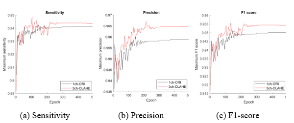
Figure 11:  Comparison of the proposed dataset (3ch-CLAHE) with the reference dataset (1ch-ORI)

The dataset with the best performance can be obtained from the experimental results in the table; however, visual performance analysis using a graph as shown in Figure 11 can be used as a tool for selecting an appropriate model and determining when to stop learning at the highest performance. The maximum measurement value (y-axis) of each epoch (x-axis) for the comparison datasets 1ch-ORI and 3ch-CLAHE appeared before approximately 200 epochs; nonetheless, stable learning results appeared after approximately 250 epochs. Two hundred and fifty epochs indicate that the learning efficiency is the best.

Figure 12 shows only a few cases among the actual detection results using the test set of 1ch-ORI and 3ch-CLAHE. Using the coordinate values of the GT box (blue box) and bounding box (green box) shown in each image, IoU was calculated and used for the evaluation.

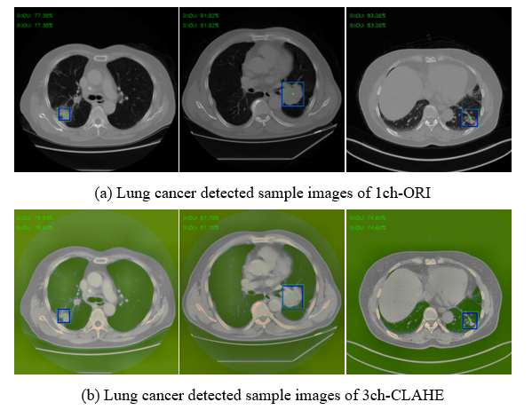
Figure 12:  Examples of detected result images

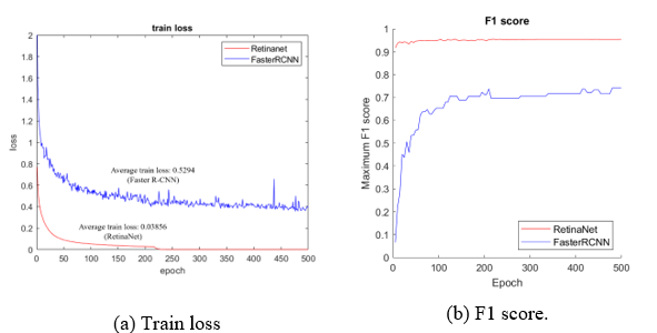
Figure 13:  Comparison of RetinaNet with the Faster R-CNN

Finally, the performance was compared to Faster R-CNN, which was used as a reference detector to select the final detector. As shown in Figure 13-(A), which compares the average train loss, RetinaNet shows a result of 0.03856. This a big difference from the Faster R-CNN, which shows a result of 0.5294, and the difference in performance and stability during the training process is reflected in the evaluation result. As shown in Figure 13-(B), RetinaNet (red line) shows a high F1-score of 0.9 or higher. However, the train loss of Faster R-CNN (blue line) is unstable, and the F1-score shows a result between 0.7 and 0.8 in Figure 13-(B).

4. Conclusion

In this study, to detect lung cancer quickly and accurately, we attempted to improve the detection performance by improving the image quality. Novel lung cancer detection methods using image processing provide a high level of accuracy by applying noise removal from CT images, segmentation techniques, and methods using 3D images for deep learning. The segmentation technique, which is mainly used to find a small nodule, has the advantage of concentrating on the area. Nonetheless, it also consumes a lot of application time and resources and has the disadvantage that the shape and boundary line may appear irregularly for each image. Because the 3D visualization method of CT images can represent the lungs more realistically, it consumes a lot of resources compared to the other methods although it is used to detect the shape of the lesion with more details.

In this study, we propose a CLAHE-based three-channel dataset construction method that automatically detects lung cancer tumors. Although this method processes CT images in a relatively simple way compared to the novel lung cancer detection methods, high performance has been confirmed through several comparative experiments, and a better performance is expected when applied to the methods of other studies.  In addition, the customization of the deep learning process is as important as the configuration of the dataset, and the experimental results reveal that the CT image with improved human visual perception is important for the neural network that mimics the human brain. However, owing to the lack of reference studies, the study was conducted with the goal of improving the performance of the original dataset, and achieved a sensitivity, precision and F1-score rates of 94.90%, 96.70%, and 95.56%. In the results of this study, the one-stage detector showed better performance in train stability and object detection rate than the two-stage detector. Since the images used in this study are medium or small size objects, different results may appear when big size objects are detected using a natural scene dataset, etc.

In addition, although this study cannot be directly compared to studies using the popular public dataset, it serves as a prior study using a dataset that has insufficient comparative studies.

5. Data Availability

The CT scan images used to support the findings of this study have been collected from the Cancer Imaging Archive (TCIA) (link: https://wiki.cancerimagingarchive.net/pages/viewpage.action?pageId=70224216)

Conflict of Interest

The authors declare no conflict of interest.

Acknowledgment

This study was supported by the Technology Innovation Program (20011875, Development of AI-Based Diagnostic Technology for Medical Imaging Devices) funded by the Ministry of Trade, Industry & Energy (MOTIE, Korea).

1. H. Sung, J. Ferlay, R.L. Siegel, M. Laversanne, I. Soerjomataram, A. Jemal, F. Bray, “Global Cancer Statistics 2020: GLOBOCAN Estimates of Incidence and Mortality Worldwide for 36 Cancers in 185 Countries,” CA: A Cancer Journal for Clinicians, 71(3), 209–249, 2021, doi:10.3322/caac.21660.
2. S. Makaju, P.W.C. Prasad, A. Alsadoon, A.K. Singh, A. Elchouemi, “Lung Cancer Detection using CT Scan Images,” Procedia Computer Science, 125, 107–114, 2018, doi:10.1016/J.PROCS.2017.12.016.
3. D. Sharma, G. Jindal, “Identifying lung cancer using image processing techniques,” in International Conference on Computational Techniques and Artificial Intelligence (ICCTAI), Citeseer: 872–880, 2011.
4. W. Sun, B. Zheng, W. Qian, “Computer aided lung cancer diagnosis with deep learning algorithms,” in Medical imaging 2016: computer-aided diagnosis, SPIE: 241–248, 2016.
5. A. El-Baz, G.M. Beache, G. Gimel’farb, K. Suzuki, K. Okada, A. Elnakib, A. Soliman, B. Abdollahi, “Computer-aided diagnosis systems for lung cancer: challenges and methodologies,” International Journal of Biomedical Imaging, 2013, 2013.
6. Y. Abe, K. Hanai, M. Nakano, Y. Ohkubo, T. Hasizume, T. Kakizaki, M. Nakamura, N. Niki, K. Eguchi, T. Fujino, N. Moriyama, “A computer-aided diagnosis (CAD) system in lung cancer screening with computed tomography,” Anticancer Research, 25(1 B), 2005.
7. K. Clark, B. Vendt, K. Smith, J. Freymann, J. Kirby, P. Koppel, S. Moore, S. Phillips, D. Maffitt, M. Pringle, L. Tarbox, F. Prior, “The cancer imaging archive (TCIA): Maintaining and operating a public information repository,” Journal of Digital Imaging, 26(6), 2013, doi:10.1007/s10278-013-9622-7.
8. P.W.S.. L.T.. L.J.. H.Y.. & W.D. Li, A Large-Scale CT and PET/CT Dataset for Lung Cancer Diagnosis, doi:https://doi.org/10.7937/TCIA.2020.NNC2-0461.
9. S. Mazza, D. Patel, I. Viola, “Homomorphic-encrypted volume rendering,” IEEE Transactions on Visualization and Computer Graphics, 27(2), 2021, doi:10.1109/TVCG.2020.3030436.
10. D. Gu, G. Liu, Z. Xue, “On the performance of lung nodule detection, segmentation and classification,” Computerized Medical Imaging and Graphics, 89, 2021, doi:10.1016/j.compmedimag.2021.101886.
11. A.A.A. Setio, A. Traverso, T. de Bel, M.S.N. Berens, C. van den Bogaard, P. Cerello, H. Chen, Q. Dou, M.E. Fantacci, B. Geurts, R. van der Gugten, P.A. Heng, B. Jansen, M.M.J. de Kaste, V. Kotov, J.Y.H. Lin, J.T.M.C. Manders, A. Sóñora-Mengana, J.C. García-Naranjo, E. Papavasileiou, M. Prokop, M. Saletta, C.M. Schaefer-Prokop, E.T. Scholten, L. Scholten, M.M. Snoeren, E.L. Torres, J. Vandemeulebroucke, N. Walasek, et al., “Validation, comparison, and combination of algorithms for automatic detection of pulmonary nodules in computed tomography images: The LUNA16 challenge,” Medical Image Analysis, 42, 2017, doi:10.1016/j.media.2017.06.015.
12. LIDC, The Lung Image Database Consortium image collection, Https://Wiki.Cancerimagingarchive.Net/Display/Public/LIDC-IDRI,.
13. I.S.G. Armato, H. MacMahon, R.M. Engelmann, R.Y. Roberts, A. Starkey, P. Caligiuri, G. McLennan, L. Bidaut, D.P.Y. Qing, M.F. McNitt-Gray, D.R. Aberle, M.S. Brown, R.C. Pais, P. Batra, C.M. Jude, I. Petkovska, C.R. Meyer, A.P. Reeves, A.M. Biancardi, B. Zhao, C.I. Henschke, D. Yankelevitz, D. Max, A. Farooqi, E.A. Hoffman, E.J.R. Van Beek, A.R. Smith, E.A. Kazerooni, G.W. Gladish, et al., “The Lung Image Database Consortium ({LIDC}) and Image Database Resource Initiative ({IDRI}): A completed reference database of lung nodules on {CT} scans,” Medical Physics, 38(2), 2011.
14. J. Ding, A. Li, Z. Hu, L. Wang, “Accurate pulmonary nodule detection in computed tomography images using deep convolutional neural networks,” in Lecture Notes in Computer Science (including subseries Lecture Notes in Artificial Intelligence and Lecture Notes in Bioinformatics), 2017, doi:10.1007/978-3-319-66179-7_64.
15. P.M. Shakeel, M.A. Burhanuddin, M.I. Desa, “Lung cancer detection from CT image using improved profuse clustering and deep learning instantaneously trained neural networks,” Measurement: Journal of the International Measurement Confederation, 145, 2019, doi:10.1016/j.measurement.2019.05.027.
16. S.K. Lakshmanaprabu, S.N. Mohanty, K. Shankar, N. Arunkumar, G. Ramirez, “Optimal deep learning model for classification of lung cancer on CT images,” Future Generation Computer Systems, 92, 2019, doi:10.1016/j.future.2018.10.009.
17. N. Khehrah, M.S. Farid, S. Bilal, M.H. Khan, “Lung nodule detection in CT images using statistical and shape-based features,” Journal of Imaging, 6(2), 2020, doi:10.3390/jimaging6020006.
18. S. Saien, H.A. Moghaddam, M. Fathian, “A unified methodology based on sparse field level sets and boosting algorithms for false positives reduction in lung nodules detection,” International Journal of Computer Assisted Radiology and Surgery, 13(3), 2018, doi:10.1007/s11548-017-1656-8.
19. TCIA, A Large-Scale CT and PET/CT Dataset for Lung Cancer Diagnosis (Lung-PET-CT-Dx) , Https://Wiki.Cancerimagingarchive.Net/Pages/Viewpage.Action?PageId=70224216,.
20. S.J. DenOtter TD, Hounsfield Unit, StatPearls Publishing, 2020, doi:10.32388/aavabi.
21. S. Ullman, R. Basri, “Recognition by Linear Combinations of Models,” IEEE Transactions on Pattern Analysis and Machine Intelligence, 13(10), 1991, doi:10.1109/34.99234.
22. Scott E Umbaugh, Computer Vision and Image Processing, Prentice Hall: New Jersey 1998, 1988.
23. O. Patel, Y. P. S. Maravi, S. Sharma, “A Comparative Study of Histogram Equalization Based Image Enhancement Techniques for Brightness Preservation and Contrast Enhancement,” Signal & Image Processing : An International Journal, 4(5), 2013, doi:10.5121/sipij.2013.4502.
24. T.Y. Lin, P. Goyal, R. Girshick, K. He, P. Dollar, “Focal Loss for Dense Object Detection,” IEEE Transactions on Pattern Analysis and Machine Intelligence, 42(2), 2020, doi:10.1109/TPAMI.2018.2858826.
25. R. Girshick, “Fast R-CNN,” Proceedings of the IEEE International Conference on Computer Vision, 2015 Inter, 2015.
26. R. Girshick, J. Donahue, T. Darrell, J. Malik, “Rich feature hierarchies for accurate object detection and semantic segmentation,” in Proceedings of the IEEE Computer Society Conference on Computer Vision and Pattern Recognition, 2014, doi:10.1109/CVPR.2014.81.
27. S. Ren, K. He, R. Girshick, J. Sun, “Faster R-CNN: Towards Real-Time Object Detection with Region Proposal Networks,” IEEE Transactions on Pattern Analysis and Machine Intelligence, 39(6), 2017, doi:10.1109/TPAMI.2016.2577031.
28. Kentaro Yoshioka, FRCNN, Https://Github.Com/Kentaroy47/Frcnn-from-Scratch-with-Keras,.
29. Young-Jin Kim, FRCNN, Https://Github.Com/You359/Keras-FasterRCNN,.
30. Yann Henon, pytorch-retinanet, Https://Github.Com/Yhenon/Pytorch-Retinanet,.
31. J. Deng, W. Dong, R. Socher, L.-J. Li, Kai Li, Li Fei-Fei, “ImageNet: A large-scale hierarchical image database,” 2010, doi:10.1109/cvpr.2009.5206848.
32. D.P. Kingma, J.L. Ba, “Adam: A method for stochastic optimization,” in 3rd International Conference on Learning Representations, ICLR 2015 – Conference Track Proceedings, 2015.

(Click Here)