1. Introduction

Vehicular Ad-hoc Networks (VANETs) are the most important element in building an intelligent transportation system and intelligent city as communication technology advances. Because VANET is a development of conventional Mobile Ad-hoc Networks MANETs, it has sparked a great deal of interest from research organizations, governments, and automakers to offer services like entertainment, consulting, information, and traffic warning; these sectors already have a lot of projects that are already started [1, 2]. According to WHO figures, 1.24 million people die globally each year as a consequence of road accidents. According to World Bank data, transportation accidents cost the global economy $500 billion a year [3]. Solving traffic congestion has become a global issue since there are more vehicles in cities. Time delays, excessive fuel usage, and environmental pollution can all be brought on by traffic congestion. In-car entertainment and vehicle-to-vehicle communication have also evolved into necessities that automakers now offer to customers in tandem with the social vehicle network [4]. Vehicle-to-vehicle (V2V) and vehicle-to-infrastructure (V2I) wireless communication are the two categories within VANETs (V2V). Many academics prefer V2V because communication is infrastructure-free, and its implementation is adaptable. VANET, on the other hand, differs from conventional MANETs in a few ways [5]. First, the network topology will frequently change in VANETs because of the fast movement of the network nodes (cars). The links are unreliable due to the short link times maintained between nodes, and vehicle distribution dramatically affects network performance. Second, car nodes are only allowed on roadways and are influenced by a variety of variables, including speed limits and traffic lights. Third, the energy constraints of VANET are no longer a significant problem because cars can generate sufficient power and computational capability for themselves. The creation of a reliable routing protocol is now a crucial step in putting VANET applications into practice as an important support technology for the realization of an intelligent transportation system. Old-fashioned routing techniques based on VANETs, such as Dynamic Source Routing (DSR), and Ad-hoc On-demand Distance Vector (AODV) [6, 7], are challenging to apply because of the frequent topology changes and poor connectivity. Since they do not take into account quick topology changes, both the transmission delay and delivery ratio are decreased for these techniques. Recently, various routing algorithms on the basis of geographic location, such as GyTAR and TFOR [8, 9], have been published [10] to address this problem. These routing techniques employ traffic flow estimates, ignore changes in topology, use GPS to find the destination node, and do not take link dependability between nodes into account. Several trustworthy routing algorithms, including EG-RAODV and SLBF [11, 12], have been presented. These algorithms were created by including characteristics like packet error rate and network dependability between nodes. Although the time delay cannot be guaranteed, this method can increase the packet delivery ratio to some amount. Rapid velocity changes are the primary cause of topology changes and faulty links in VANETs. Good evaluation of connection dependability and effective routing algorithm designs can only result from a thorough understanding of vehicle motion characteristics. Assuming that cars are traveling along a set path, a number of variables, including the two vehicles’ directions of travel, their distance from one another, their speeds, and their acceleration, can cause a link to be severed between two nodes. Given the low-density, high-speed environment, these aspects must be completely considered in evaluating connection reliability between nodes properly. When maintaining traffic safety and assessing link reliability, the space between vehicles is crucial. Many models of vehicle separation, including the log-normal distribution, the normal distribution model, and the exponential distribution model, have been put forth. In [13], the authors used tests to demonstrate that when the distance between vehicles follows a log-normal distribution, It may be more in line with the way traffic really moves and with safe separations. Effective evaluation of link dependability between nodes requires a thorough grasp of the moving characteristics of moving objects and the traffic flow model. Routing algorithms have been the subject of continuing research, and VANETs have used several efficient algorithms [14] and have outperformed conventional routing algorithms. Q-Learning [15] is a self-learning algorithm that may continuously interact with its surroundings to find the shortest route from a source node to a destination node. This research improves upon the Q-Learning method and suggests a new technique for adaptive routing that is both efficient and trustworthy. It may adaptively modify the Q-table while guaranteeing the dependability of each hop connection, allowing it to conform to changing network architecture like that of a VANET. This paper’s major goal is to provide a trustworthy and flexible routing algorithm. The links between each hop determine how reliable a link as a whole is. By carefully examining the motion characteristics of cars, this work creates a trustworthy model of a link between nodes. Once the probability of link dependability has been determined, the Q-Learning algorithm can use it as a parameter to create the RSAR algorithm.

In the first section, the routing method is categorized and then partially explored in the second section. In the third part, we discuss how to create an accurate model for evaluating reliable links. The fourth and fifth section consecutively addresses The RSAR algorithm’s fundamental idea and the simulations and analysis that were done. A summary and recommendations for further work are given in the sixth and last sections.

2. Proposed solution

2.1. Q-learning algorithm in VANETs

Standard Q-Learning is an agent-based heuristic learning technique. The three-tuple R, S, and A make up the majority of the learning process for the agent in the widely used Q-Learning algorithm. Where R denotes the instant reward for an action, A ={a1,a2,⋯,an } the activity space, and S ={S1,S2,⋯,Sn } denotes the state space. The larger the reward gained for the action, the nearer the agent is to the target. The learning process will be thoroughly explained in the following subsections once a few related definitions are presented.

• Definitions

• Fundamental elements.

The whole VANET environment is used by the agent as its learning environment.

Learning Agent: Each node of the vehicle functions as its own independent learning agent;

State space (S): All nodes other than this agent make up the state space of a specific agent;

Activity space (A): An activity is the transmission of a beacon packet between two vehicles;

Immediate Reward (R): The instant reward that is given to an agent once they have successfully completed an activity.

2.2. Value of a reward

The instantaneous reward, which has a range of [0,1] and is the reward received by an agent after performing an action, is defined in Definition 1. The reward value for the destination node is 1, as it can directly contact the destination node. Formula (1) specifies the beginning value R of the whole network as follows:

 Stands for the set of destination node D’s one-hop neighbor’s node; the reward value of an action is 1. The Q-value , , which is in the range [0,1], stands for the potential reward value that is earned while moving from one learning stage.

Q-table definition: Every learner maintains a two-dimensional table with the Q-values of the nodes it can reach and its immediate neighbors. The Q-table is a two-dimensional table (see Table 1).

Table 1: Q-table

	D1	D2	…
N1	Q(D1,N1)	Q(D2,N1)	…
N2	Q(D1,N2)	Q(D2,N2)	…
…	…	…	…

The IDs of every potential destination node are written as  In the first line of the Q-table. The one-hop neighbor nodes’ IDs, denoted as , are listed in the first column. The value of  represents the Q-value between the sending node and its neighbor N1 at the receiving node . As can be seen in Table 1, the size of the Q-table is dependent on both the number of destination nodes and the number of neighbor nodes. One can see that it can be climbed with relative ease.

Beacon packets are periodically exchanged between nodes to update the values in the Q-table. Each node receives a share of the learning task, which causes the algorithm to swiftly find the best path and allows for prompt adaptation to network topology changes.

2.3. Learning process

The aforementioned definitions established each vehicle node as a learning agent. An individual Q-table is associated with each vehicle node, in contrast to conventional learning methods. Nodes complete their learning process by sharing beacon data and updating their Q-tables.

Along with its own speed, position, and other information, each node additionally includes the maximum Q-value of the nearby nodes to the destination node, or the greatest value in a column, in the beacon packet it transmits (as shown in Table 2). Given a VANET topology,   , as shown in Figure 2, we assume that the state space of node A is the series of all nodes that don’t include A. The collection of vehicle nodes is represented by . The set E of edges characterizes a collection of connected nodes that may exchange messages with each other with a single additional hop. As depicted in Figure 3, let’s pretend that from node A, we go to node G as the endpoint. The goal now is to use a self-learning algorithm to determine the best route from node A to G, where A is the starting point.

Each vehicle node agent is given learning tasks, and as part of the learning process, the agent’s Q-table and the state activity Q-values, , are primarily updated.

Table 2: Network parameter settings

Parameter	Value
Size of topology (m*m)	3511m*3009m
Video file frame size	30 fps
Image Resolution	352 * 288
CBR packet size (bytes)	512
Simulation time (s)	300
Propagation model	Two-ray ground
Transmission range	250
MAC standard	IEEE 802.11 MAC (2 Mbps)

Eq. (2) contains the usual Q-Learning function:

R is the reward value, D represents the destination node,  is ‘s neighbor node, x is its neighbor node, S is the node to go from node x to node D, the maximum Q-value between x and its neighbor is  max y E n.

The reward a node gets for completing an action in accordance with Eq is impacted by the discount factor , making it a significant parameter (2). Since link stability is an essential factor, we used the between-node link reliability r, calculated using Eq. (15) as a discount factor; thus, r = r. (l). The pace of packet transmission in VANETs is a critical metric that depends on the available bandwidth.

The definition of the bandwidth  BW is as follows:

where  Is the packet size in bytes,  is the time interval, and packets sent and received by the node are denoted as n. With the assumption that the node’s maximum bandwidth, denoted by max BW, is a constant Here’s how you can figure out your bandwidth:

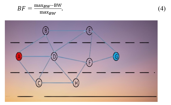
Figure 1: Learning process

Each vehicle node’s learning progress is determined by the bandwidth factor. It fluctuates as the element that affects learning speed, depending on variations in effective bandwidth. A new heuristic function can be produced by changing equation (2):

According to Eq. (5), as the hops number rises, the reward value drops. The final reward value depends on the bandwidth, the dependability of the network, and the number of hops. In a dynamic network, By combining bandwidth and connection state, the most efficient path may be determined between the source and the destination node. The destination node G’s one-hop neighbors in Figure 1 are nodes F and E. According to Eq (5),  and  are the appropriate representations for the reward values from nodes E & F to the destination node G.

It is possible to determine that the ultimate Q-values of  and  are 0.7 and 0.8, respectively, after accounting for the impacts of bandwidth and link quality. A, B, C, E, F, and H are D’s nearby nodes. When node D receives a beacon packet from any neighbor, it processes the packets and extracts the maximum Q-value to node G by using F, . Calculate the relevant Q-value, or  In accordance with Eq. (5) and update the Q-table.

Being the largest,  will have a value of 1 within the beacon packet. Data packets from other nodes will go through the same processes, after which a selected column in the Q-table will be updated. As shown in Figure 2, the remaining neighbor nodes’ Q-tables are changed such that    in compliance with Eq (5). The maximum Q-value between node D and its neighbors is updated in real-time by node D’s Q-table as neighbor data packets are constantly received. In a similar vein, when node D transmits a beacon packet, it looks for the maximum Q-value among itself and its neighbors in a certain column of the Q-table. As soon as node A receives the beacon packet from node D, it will send the highest possible Q-value and continue the calculation to update QA. The same procedure is employed when additional nodes send in beacon packets. The outcomes depicted in Figure 4 will ultimately be attained by continuous data packet exchange [16,17].

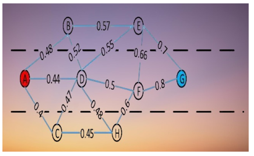
Figure 2: Q-values to the destination node G saved by each node

The best route from A to G may be easily identified, as shown in Figure 2. The best route is the one with the highest Q-value of its nodes. As seen in Figure 4, the best path is ABEG since it has the highest Q-value. The dynamic update-and-save of the Q-table allows the method to quickly, consistently, and robustly react to topology changes.

2.2. The proposed RSAR algorithm

2.2.1. Transmission process

The three actions listed below are carried out by the RSAR algorithm when it routes data packets:

Step 1. Node A checks its internal Q-table before sending a data packet to Node B to see whether Node A is the next hop for Node B. If not, it begins the route development process, which is covered in the next subsection; when this is the case, it picks the node nearest to it that has the greatest Q-value.

Step 2. At the point when the route has been constructed, the fundamental path from the starting node to the ending node has been determined, and the necessary vehicle nodes have been learned. We initiate the route maintenance operation to dynamically keep the end-to-end connection up and running, which is necessary for finding the best path across the whole network topology and resolving the segmentation problem. The next subsection details the route maintenance procedure.

Step 3. The aforementioned procedures establish the best route for the overall network topology. A vehicle node will carry out the first step if it receives or sends data packets; If not, it will proceed to step 2.

2.2.2. Route development and Maintenance Process

Before sending data, a node checks its internal Q-table to determine whether there is a next-hop node between it and the destination. The data packet is sent to the neighboring node with the highest Q-value relative to the target node. If there isn’t one, route discovery is initiated. A path request timer is started at the source node, which subsequently sends out a req packet to the entire network. Within the req data packet, the source node keeps a record of the IDs of all of the nodes that the data packet traveled through while it was being routed across the network. The rep packet is saved by the destination node once it has received it for the first time from the source node. Subsequent rep packets received by the destination node are deleted. After extracting the ID information that it recorded from the rep data packet and flipping it, the node at the end of the route creates a data packet labeled req and stores the reversed path information there. Finally, the req data packet is discarded. After waiting for an open time window, it sends the req data packet via the recorded reverse route. Upon receipt, a node that has been previously recorded will make the necessary adjustments to the data packet’s next hop address, refresh its Q-table, and then broadcast the packet using a single hop. When the packet is received by other nodes that are not the destination, those nodes will just alter their Q-tables and then discard the packet. The source node will suspend the request timer as it works on updating its Q-table while waiting for rep to be transmitted to the destination node, it also serves as the req source node. At this step, a route from the source to the destination node has been identified, and the Q-tables of the nodes on the first path are modified; their starting values are 0.

The values of the Q-tables of some of the nodes that are adjacent to the initial route path are also updated when that path is constructed. It is essential to get the process of route maintenance going as soon as possible in order to guarantee that the path will continue to be useful despite the dynamic changes in the network [18,19]. The maintenance of the Q-tables in a dynamic manner and the resolution of the issue of network segmentation are the primary goals of the process of route maintenance. Each node will, at regular intervals, broadcast beacon packets in order to keep the Q-tables of its neighboring nodes up to date. The beacon data packet will primarily provide the node’s position, speed, and maximum Q-to-Value ratio.  – Value  was discussed in conjunction with the method of education. In the experiment, the beacon packet’s transmission delay was set to a random value between [0.5, 1], which was done to guarantee that the update would be effective. For the sake of the Q-table, the actual time at the destination node has been supplied. When a destination node’s time hasn’t been changed for more than the specified length of time, the data column associated with it is deleted, and the destination node is deemed invalid. In the event of a network split due to a moving vehicle, RSAR initiates the route request timer and makes use of the store-and-forward method to ensure that an R-req data packet is transmitted. In the event that the sending node sometimes doesn’t receive the R-rep data packet from the receiving node before the timeout expires, the receiving node is considered inaccessible, and the transmission is aborted. Failure to do so will result in the routing route being restored at the point of disruption.

3. Experimental tests

3.1. System Model

As stated in [20, 21], it is reasonable to assume that the highway is often a straight road and that the broadcasting distance is much greater than the width of the road, both of which are necessary for an accurate evaluation of the connection quality between nodes. The road’s width may also be assumed to have negligible effects on forwarding node selection at the following hop and, therefore, may be disregarded. This is essential in order to accurately gauge the quality of inter-node connections. As shown in Figure 3, the simulated highway was created using the above methods.

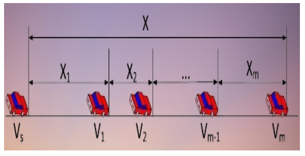
Figure 3: Road model

It is also reasonable to presume that other maneuvers, like speeding up and slowing down, switching lanes, passing other vehicles, and so on, are taking place on the roads. In addition, the distance that separates cars follows a log-normal distribution [22,23], which can be written as  A random variable with a log-normal distribution is depicted in Figure 1 as , where m can take the values 0, 1, or 2.  denotes the distance between vehicles  and and  denotes a random variable at moment m, representing the distance between node I and its related nodes. If the node  in Figure 1 is considered to be the reference node, then the value  reflects the distance between  and any other node. Since X denotes the distance between other nodes and  , and X is also log-normally distributed.

Proposition 1: Let’s assume that  and that the variable  is log-normally distributed, where    and .

If the probability distribution function of the t is Then, for each positive . Apparently, as  is continuous,

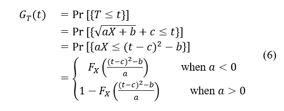
 is the probability distribution function of . When a>0, it is evident that T follows a log-normal distribution. When , according to [13], And letting

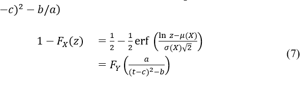
 is a log-normal random variable with parameters  and . Since the fact   is used. Consequently, T conforms to a log-normal distribution, concluding the proof.

The direction of motion is indicated by the black arrows in Figure 2, where two cars are shown in “a” going in the same direction, whereas two vehicles are depicted in “b” moving in the opposite way.

Proposition 2: Assuming that ,  is log-normally distributed, where  and ,  (The reasons offered in the proof of 1 may be used to simply demonstrate this)

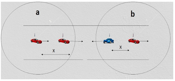
Figure 4: Two cases of link breakage

There are two basic circumstances (shown in Figure 4) in which the connection between two nodes breaks if we assume that the cars are traveling along a fixed route. Both of the vehicles depicted in Figure 4a are moving in the same direction, whereas both of the vehicles depicted in Figure 4b are progressing in opposing directions. Think of vehicle i as the transfer point and vehicle j as the reference point in this scenario. Under normal circumstances, the longest communication durations between vehicles occur between i and j. The next thing that needs to be done is a comprehensive analysis of the link duration for these two different scenarios.

At time , if the car i is in front of car j, then car i can communicate with car j with just one-hop. This is demonstrated in Figure 4a.

A random variable will be used to determine the initial distance between vehicle X. There is not going to be any change in the maximum communication radius of vehicle R. X fulfills these conditions at the outset:

On a highway, there will reportedly be instances of accelerating, decelerating, and passing other vehicles in accordance with the system model. On this stretch of road, the maximum speed limit is , which means that all vehicles must travel at a speed that is either lower than or equal to . Consider the fact that the vehicle is moving at a speed of  and that its acceleration is .

When time is less than zero, the acceleration is denoted by the symbol , and the speed is denoted by the The acceleration, as measured at time t, is calculated as follows:

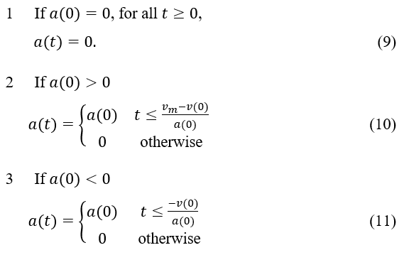
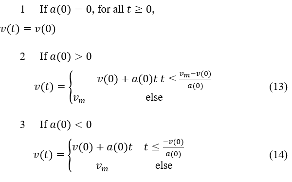
Based on the analysis presented above, it is reasonable to conclude that when , assuming that the current acceleration  is zero, the instantaneous acceleration would be 0 as well,  which is denoted by the equation . If the speed is less than (0) the maximum speed limit, the acceleration is presumed to be ; if the speed is more than the maximum speed limit, the acceleration is set to 0. If the speed is above the maximum speed limit, it is changed to 0. Taking into consideration the speed at the beginning, , the instantaneous speed, , can be defined by the following formula at time t:

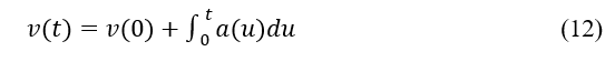
where  is the acceleration at time .

The instantaneous speed may now be calculated by combining Eqs. (6-9):

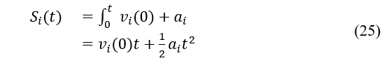
The following formula can be used to calculate the distance traveled by any vehicle traveling at a speed of  during the interval of time represented by [0, t]:

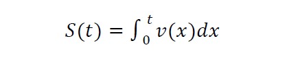(15)

Again, in accordance with the definition presented above, it is possible to determine the gap in space that exists between vehicles i and j at a particular instant in time, as shown in Figure 4.

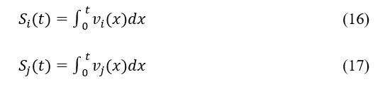
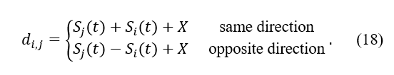
If we assume that the initial acceleration and  speed of i and j vehicles are, respectively , and vj(0), then the instantaneous acceleration and speed of vehicles i and j at time t are, respectively , and . The following equation can be used to determine the distance between the cars I and j at the time [0, t] if Eqs. 9–15 is followed to their logical conclusions:

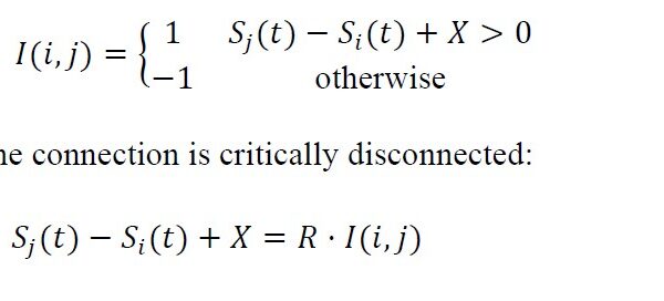
If the distance between vehicles i and j at the beginning of the race is X, the distance  between those two vehicles at the end of the race is:

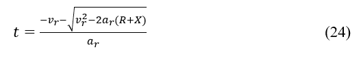
The conclusion that the link is severed can be drawn from Equation 13, which states that when , the connection is severed. The following thing that needs to be done is an analysis of the link duration in Figure 2b. This demonstrates how two automobiles meet while traveling in different directions:

Now it is possible to determine the maximum link duration t. We can calculate the maximum link duration t as follows using the assumption that , where  and .

If two vehicles are going in the same direction, as shown in Figure 2a, determine which one is in front by overtaking, decelerating, and accelerating. Vehicle j is in front of vehicle i when ; conversely, vehicle i precedes vehicle j. A symbolic function was defined as follows to efficiently convey which car is in front:

To compute the link duration at this time, two cases must be taken into account.

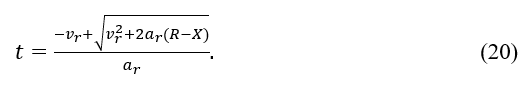
When , vehicle j is in front of vehicle i. From Eq. (20), . Similarly, to Eq. (20), because , where  and   The time  can be determined as:

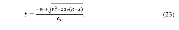
The position of vehicle i in relation to vehicle j is the same when .  and the link duration t may be calculated from Eq. (1) as follows:

To calculate the link duration between two nodes within a one-hop range: the transmitting node and the other nodes utilize equations (20), (23), and (24).

Proposition 3: If vehicle i and j’s communication link fails at time t, the remaining link duration is a linear or square root function of X.

Proof: It is known that, at a constant speed ,   is a linear function of t, i.e., , based on the definition of S i (t) according to Eq. (15), which happens after the connection is lost at time t. S i (t) = at + b. Similarly, it may be inferred that  is a linear function of t if  is a constant. Eq. (23) clearly states that  when the two cars are moving in different directions. The linear function for the link duration time is . Once a connection is made between two co-directional vehicles i and j, the link duration is also a linear function, as shown by the equation . As a result, when  and  are both constants, and the link duration t is a linear function. A quadratic polynomial will represent the distance function if either  or  are not constants. Allow     without losing generality. The distance function is, by definition:

Eqs. (14) and (22) demonstrate that  . Consequently, the answer is a square root function of X.

First Theorem Vehicles i and j’s link’s duration T have a log-normal distribution.

Proof According to Proposition 3, the connection duration can be written as  or . The expression  is log-normally distributed according to Proposition 1.  is distributed log-normally according to Proposition 2. As a result, the link’s duration always follows a log-normal distribution. The theorem’s proof is now complete.

The link duration of the cars i and j is log-normally distributed as , where the variance is  and expected is Based on the link duration between the nodes. The duration of the link may then be used to assess its dependability. The likelihood of two vehicles directly communicating throughout the time period . is known as link reliability. When The connection dependability between nodes is, supposing that any two vehicle nodes have a communication link :

where the probability function for the time period T is expressed by f(T).

• 2. Simulation setup

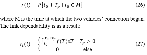
As seen in Figure 5, the experiment was simulated using NS-2 and a 3511m*3009m square topology using a real-life map of “ Anfa District in Casablanca.” The topology included intersections and straight roads, each of which had been built up with two-way lanes. To add authenticity to the simulation, each vehicle node in the network employed an intelligent driving model (IDM) that featured waiting, avoiding, overtaking, and lane switching.

The default NS-2 parameter settings are shown in Table 2. we have used a CIF (H.261) video file format with a 352 x 288. UDP was utilized for transmission following the work approach shown in Figure6.

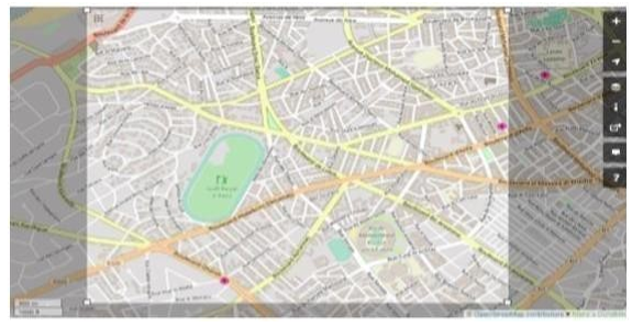
Figure 5: Anfa District Casablanca “OpenStreetMap”

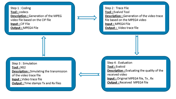
Figure 6: Work approach

In contrast with the Enhanced Distributed Channel Access (EDCA) defined in the 802.11p standard, the video transmission was carried out using an Enhanced Dynamic Cross-layer mechanism for real-time HEVC streaming. This method has proven to deliver improved performance in video quality at reception and end-to-end latency. QoS and QoE calculations have been in use for the verification of the effectiveness of the cross-layer mechanism shown in Figure7 in a separate paper.

Figure 7: Illustration of the Adaptative mapping algorithm.

Each beacon packet’s size was determined based on the data that was transmitted. Two scenarios that simulated the scenario in Figure 5 were put up to successfully assess the RSAR algorithm’s performance. The first scenario used a network with 80 nodes and vehicle peak speeds between 30 and 90 kilometers per hour. In this case, we will focus on how the speed of the vehicle impacts the routing protocol and provide an explanation. The alternative scenario went as follows: the cars’ top speed was fixed at 40 km/h, and there was anything between 60 and 120 nodes. The discussion in this instance will center on how vehicle density affects the routing protocol. The nodes were first scattered at random along several roadways and followed a predetermined path.

Each simulation was repeated 20 times with an average value of 300 s between each run. The simulation data were then assembled.

3.3. Simulation results

The QLAODV algorithm, the SLBF algorithm, the GPSR algorithm [11, 14, 17], and the techniques described in [22, 24] were contrasted with the RSAR algorithm suggested in this study. All of these algorithms are examples of routing algorithms. It is feasible to assess the benefits and drawbacks of RSAR thanks to this comparison. The results illustrated in Figs.  8, 9, 10, 11, 12, 13, and 14 were acquired by comparing end-to-end delays; the packet delivery ratios hop number in various scenarios. Figures 8, 9, and 10 show the comparisons of the first test, while figures 11, 12, and 13 show the comparisons in the second test case.

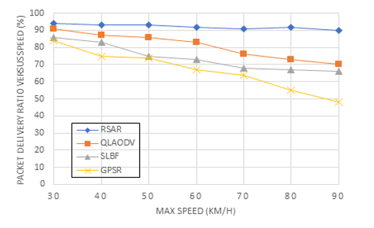
Figure 8: Packet delivery ratio on different speeds

Figure 8 shows that there is a direct association between the speed and packet delivery ratio. A node’s packet delivery ratio is calculated by data packets supplied by that node by the data packets received by the destination node. Figure 8 demonstrates that the RSAR suggested in this paper was able to achieve a consistent and high packet delivery ratio of video data; as speed increased, the average ratio up surged to more than 90%. With increasing speeds, the packet delivery ratios of the other three investigated routing methods dropped dramatically. This enhancement was made possible thanks to RSAR’s careful consideration of how to speed variations affect link reliability. The Q-Learning method uses this information as a learning parameter to make routing decisions by analyzing the links between nodes and determining the dependability of those links. Due to its greedy approach and lack of consideration for connection reliability, while choosing the next hop node, GPSR’s packet delivery ratio decreased quickly. Until the speed reached 54 kilometers per hour, QLAODV’s packet delivery ratio was over 90%, but it rapidly dropped after the speed was exceeded. QLAODV, although using the Q-Learning paradigm, must constantly repair the route with increasing velocity to provide an always-reliable path from beginning to finish. As a result, the proportion is reduced. Due to its sensitivity to topology changes, SLBF’s packet delivery ratio decreased and does not take connection stability into full account. It was more similar to the GPSR algorithm because it used a greedy approach.

Figure 9 shows the connection between speed and end-to-end time delay; In this case, the time delay is measured as the typical amount of time it takes for the receiving node to receive a valid data packet. Figure 9 shows that when the vehicle nodes’ speed rose, all four techniques’ time delays showed a growing trend. The RSAR algorithm suggested in this paper had a rather constant time delay that fell between SLBF and GSPR. When the maximum speed was greater than 60 km/h, the time delay of SLBF quickly grew and surpassed that of RSAR. The effects of topology modifications and the requirement for a new computation of the re-transmission method or effective forwarding area were the main causes of this trend. While topological modifications have less effect on RSAR, this method ensures that the route with the best Q-value has the most available bandwidth, the least unreliable connection, and the shortest routing distance. Because GPSR solely employs the greedy forwarding method, its time delay was the shortest. The GPSR had the lowest packet delivery ratio since it exclusively employs the greedy mechanism, dropping packets as soon as they don’t arrive. Although QLAODV also employs the Q-Learning model, its increased speed requires frequent path switching in order to maintain an efficient routing path.

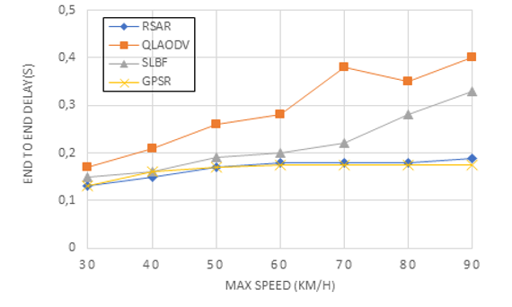
Figure 9: End-to-end delay on different speeds

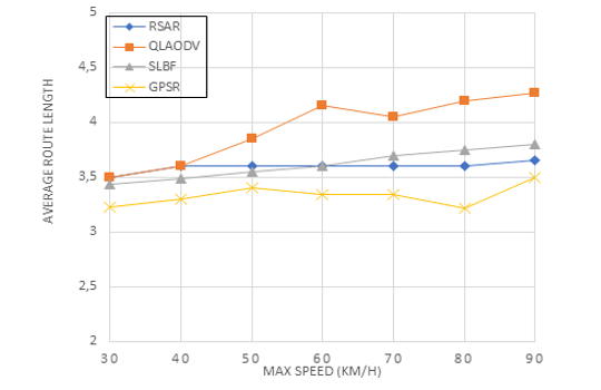
Figure 10: Routing length on different speeds

This resulted in a significant lengthening of the packet delivery time. According to Figure 9, in the context of a topology that was rapidly changing, the RSAR packet delivery ratio ranged from 0.1 to 0.2.

Figure 10 shows the relationship between speed and route length using the average number of hops required by valid data packets to reach their destination. Rather than relying on a route transformation mechanism to ensure that the whole path is maintained, this approach employs a simple forwarding decision to determine which node has the greatest Q-value; as shown in Figure 10, RSAR’s route length was less than that of QLAODV. The RSAR suggested in this paper has a consistent route length, as seen in Figure 10. The maximum Q-value and store-and-forward selection mechanisms make this feasible by always using the shortest route possible. Both GPSR and SLBF use a greedy packet forwarding strategy, however when the speed increases over 60 km/h and topological changes become more pronounced, SLBF’s route length increases; despite the fact that GPSR employs no trustworthy technique, the lowest number of hops was reached.

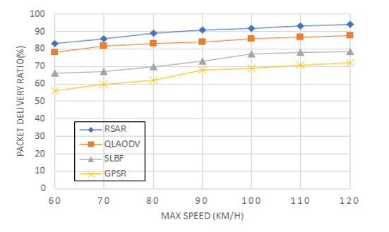
Figure 11: Packet delivery ratio by number of nodes

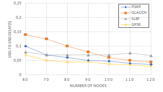
Figure 12: End to end by the number of nodes

The relationship between packet delivery ratios and the number of nodes is seen in Figure 11. Overall, the packet delivery ratio improves with increasing network size across all four approaches as the number of nodes increases. Over 90% packet delivery ratio is achieved in RSAR with 90 nodes, while the packet delivery ratio for QLAODV is 85%. RSAR fully takes into account connection stability between nodes despite the fact that both of these algorithms are based on the Q-Learning concept, which results in a significantly higher packet delivery ratio. The store-and-forward mechanism makes RSAR’s packet delivery ratio superior to that of GPSR and SLBF in the presence of a growing number of nodes. As SLBF employs the retransmission technique, it has a higher packet delivery ratio than GPSR, but because topology has a significant impact because the sending node and vehicle are frequently on different paths, it has a lower packet delivery ratio than RSAR.

Figure 12 describes the link between the end-to-end time delay and the number of nodes. The RSAR’s end-to-end latency is quickly catching up to the GPSR’s. This is because when nodes are added, RSAR learning nodes are also created, reducing the time delay and shortening the route to the target node. The time delay of QLADOV eventually approaches that of RSAR as the number of nodes rises, but with fewer nodes, it is significantly bigger than that of RSAR. As QLAODV spends so much time maintaining the routes, this behavior arises. Because it employs a scheduled broadcast technique that causes an increase in time delay, SLBF drops slowly with an increase in the number of nodes. As the number of nodes rises, the time delay for each of the four algorithms decreases.

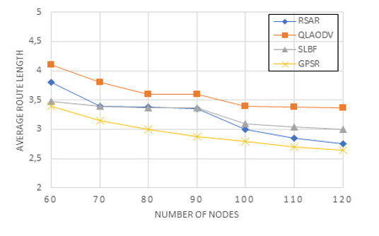
Figure 13: Routing length versus the number of nodes

Figure 13 shows the association between the number of nodes and the average route length. The average route length of all four techniques decreases as the number of nodes rises. The primary reason for this is an increase in the number of effective forwarding nodes. RSAR’s route discovery is shorter than QLAODV’s path discovery. As GPSR and SLBF both employ a greedy strategy, the path lengths of GPSR, SLBF, and RSAR are near to one another. RSAR chooses the next hop that is closest to the furthest node as the number of nodes increases.

3.4. Summary and discussion

As seen in the previous section, the simulation was based on the two factors that affect the most quality of video transmission those are Speed and the number of nodes.

When speed increases, we have determined that in terms of packet delivery ratio, RSAR was able to achieve a high and consistent packet delivery ratio of video data, with an average ratio of more than 90%, as speed increased. In terms of end-to-end delay, the RSAR algorithm had a rather constant time delay that fell between GSPR and SLBF. In terms of route length, RSAR’s route length was less than that of QLAODV, thanks to the maximum Q-value selection and store-and-forward mechanisms.

In terms of packet delivery ratio, we have concluded that when the number of nodes increases, RSAR kept a ratio above 90%, while the packet delivery ratio for QLAODV was around 85%. In terms of end-to-end delay, The RSAR steadily approaches the GPSRs thanks to the fact that when nodes are added, RSAR’s learning nodes are added as well, making the path to the time delay and destination node shorter. Each of the four approaches has a reduced average route length as the number of forwarding nodes increases.

4. Conclusion and future work

In this research, a reliable adaptive routing service method is suggested to address the issues of dramatic topological changes and unstable links brought on by quick vehicle movements in VANET. First, it was established that links had a log-normal distribution in terms of duration after studying the characteristics of vehicle motion and the causes of links’ lack of reliability. Second, a link reliability calculation model was created using this information. After the link reliability between nodes was evaluated as a parameter and employed in the Q-Learning process, the RSAR method was then recommended. The effectiveness of four routing methods was then evaluated using simulated trials to measure the number of hops, packet delivery ratios, and end-to-end delays. Under varying circumstances, the findings demonstrated that RSAR achieved a greater packet delivery ratio with a shorter transmission time delay. Due to its self-learning capabilities, RSAR is well-suited to deal with the issues caused by topological changes. Local diffusion is a kind of technique used in learning, and there may be a huge number of nodes involved in choosing the route, so the routing cost in a big network environment will be quite high. As a result, the authors’ future work will concentrate on the issue of routing expense.

The creation of the algorithm that was used in finishing tracks at the MAC layer while meeting low latency requirements. Due to the time limit, packages that are not received by the recipient within the time limit do not count towards the total duration of the film. This is done in order to maintain the integrity of the timeline. Because of this, their transmission is completely worthless and does nothing more than burden the network. This feature of the algorithm must be taken into account, as eliminating them at the transmitter would enhance transmission. The technique should form a relationship between the application time constraint, the round-trip time limit, and the transition time represented by the completion of the waiting list to be considered valid.

1. M.G. W.L. Junior, D. Rosário, E. Cerqueira, L.A. Villas, “A game theory approach for platoon- based driving for multimedia transmission in VANETs” , Wireless Communications and Mobile Computing, 2414658, 1–11, 2018, doi:https://doi .org /10 .1155 /2018 /2414658
2. A.V.V. M. Jiau, S. Huang, J. Hwang, “Multimedia services in cloud-based vehicular networks” , IEEE Intelligent Transportation Systems Magazine, 7 (3), 62–79, 2015, doi:https://doi .org /10 .1109 /MITS .2015 .2417974
3. X.Z. M. Gerla, C. Wu, G. Pau, “Content distribution in VANETs”, Vehicular Communications, 1(1), 3–12, 2014, doi:https://doi.org/10.1016/j.vehcom.2013.11.001
4. R.S. C. Campolo, A. Molinaro, “From today’s VANETs to tomorrow’s plan-ning and the bets for the day after”, Vehicular Communications, 2 ( 3), 158–171, 2015, doi:https://doi .org /10 .1016 /j .vehcom .2015 .06 .002
5. R.F.S. D. Perdana, “Performance comparison of IEEE 1609.4/802.11p and 802.11e with EDCA implementation in MAC sublayer”, International Conference on Information Technology and Electrical Engineering (ICITEE), 285–290, 2013, doi: 10.1109/ICITEED.2013.6676254
6. N. Mittal, A. Singh, “A Critical Review of Routing Protocols for VANETs” , International Conference on Innovative Computing and Communications, Springer Nature Singapore Pte Ltd, 135-142, 2019, doi: doi.org/10.1007/978-981-13-2324-9_14
7. F. Goudarzi, H. Asgari, and H. S. Al-Raweshidy, “Traffic-Aware VANET Routing for City Environments—A Protocol Based on Ant Colony Optimization”, IEEE SYSTEMS JOURNAL, 1-11, 2018, doi: 10.1109/JSYST.2018.2806996
8. IEEE P1609.4, “Trial-Use Standard for Wireless Access in Vehicular Environments (WAVE) — Multi-Channel Operation ”, IEICE transactions on fundamentals of electronics, communications and computer sciences, 12 (2010), 2691-2695, 2006.
9. S. ZAIDI, “Le streaming vidéo dans les réseaux véhiculaires ad-hoc,” Doctoral thesis, UNIVERSITE MOHAMED KHIDER- BISKRA, 2018, doi : http://thesis.univ-biskra.dz/id/eprint/3870
10. M. Rouse, “Vehicle-to-vehicle communication (V2V communication)” , Internet of Things Agenda, 2014, doi : https://doi.org/10.48550/arXiv.2102.07306
11. M. Zorkany, N.A. Kader, “Vanet routing protocol for v2v implementation: A suitable solution for developing countries” , Cogent Engineering, 4(1), 1362802, 2017, doi : https://doi.org/10.1080/23311916.2017.1362802
12. S. Chakrabarti, L. Technologies, A. Mishra, V. Tech, “QoS Issues in Ad Hoc Wireless Networks” QOS and resource allocation in the 3rd generation wireless networks, IEEE, 142-148, 2001, doi : 10.1109/35.900643
13. G. Ya, S. Olariu, “A probabilistic analysis of link duration in vehicular ad hoc networks”, IEEE Intelligent Transportation Systems Magazine, 12 ( 4), 1227-1236, 2011, doi : 10.1109/TITS.2011.2156406
14. J. Toutouh, “Intelligent OLSR routing protocol optimization for VANETs”, IEEE Transactions on Vehicular Technology, 61(4), 1884-1894, 2012, doi : 10.1109/TVT.2012.2188552
15. YN . Zhu, “A new constructing approach for a weighted topology of wireless sensor networks based on local-world theory for the internet of things (IOT)”, Computers & Mathematics with Applications, 64 (5), 1044-1055, 2012, doi : https://doi.org/10.1016/j.camwa.2012.03.023
16. YP . Liang, “ A kind of novel method of service-aware computing for uncertain mobile applications”, Mathematical and Computer Modelling, 57 ( 3–4), 344–356, 2013, https://doi.org/10.1016/j.mcm.2012.06.012
17. XD Song, X Wang, “ Extended AODV routing method based on distributed minimum transmission (DMT) for WSN”, AEU – International Journal of Electronics and Communications, 69(1), 371–381, 2015, doi : https://doi.org/10.1016/j.aeue.2014.10.009
18. Z Ke, Z Ting, “ A novel multicast routing method with minimum transmission for WSN of cloud computing service”, Soft Computing, 19(10): 1817-1827, 2015, doi : https://doi.org/10.1007/s00500-014-1366-x
19. XD Song, X Wang, “ Extended AODV routing method based on distributed minimum transmission (DMT) for WSN”, AEU – International Journal of Electronics and Communications, 69(1), 371–381, 2015, doi : https://doi.org/10.1016/j.aeue.2014.10.009
20. T Saravanan, N.S. Nithya, “ Modeling displacement and direction aware ad hoc on-demand distance vector routing standard for mobile ad hoc networks”, Mobile Networks and Applications, 24(9), 1804–1813, 2019, doi : https://doi.org/10.1007/s11036-019-01390-9
21. T Saravanan, N.S. Nithya,” Energy aware routing protocol using hybrid ANT-BEE colony optimization algorithm for cluster based routing”, 4th IEEE ınternational conference on computing communication and automation (ICCCA), 1–6, doi : 10.1109/CCAA.2018.8777662
22. P Sherubha, N Mohanasundaram, “ An efficient network threat detection and classification method using ANP-MVPS algorithm in wireless sensor networks”, International Journal of Innovative Technology and Exploring Engineering (IJITEE), 8(11), 2278-3075, 2019, doi : https://www.ijitee.org/wp-content/uploads/papers/v8i11/F3958048619
23. V. Tavares, J.M.R.S. Boulogeorgos, A.A.A. Vuppalapati, “ International Conference on Communication, Computing and Electronics Systems”, Lecture Notes in Electrical Engineering, Springer, Singapore, 733, doi : https://doi.org/10.1007/978-981-33-4909-4_60

(Click Here)