1. Introduction

This paper is an extension of the work that was originally presented at the 2021 International Conference on Electromechanical and Energy Systems [1], which was referring to the sizing of components and design of control systems that can be applied in an MG primary control layer powered by solar energy in Ecuador.

Verifiably, one of the principles of large-scale electricity generation is the installation of generators in areas close to energy resources, such as thermoelectric power plants near natural gas deposits. Listing some disadvantages, energy resources are usually non-renewable in several power generation projects, and typical installations are inappropriate when final consumers are far from power plants. Due to these remote destinations, infrastructure costs would rise, this being the construction of one or more substations to mitigate voltage drops in distribution cables.

Several agricultural production farms are in different inaccessible areas along the Ecuadorian coast, which has led several producers to use diesel pumps for irrigation systems. Due to recent studies and the acceptance of PV plants in Ecuador, it is possible to provide a solution with PV MGs for final loads found in distant destinations such as pumps and small residential consumption.

Concurring to a few definitions, an MG is a local and small energy system that can function in a connected mode to the main grid or a self-regulating disconnected mode. It is made up of several distributed energy sources that supply heterogeneous loads within clearly defined electrical boundaries and by a variety of control criteria [2].

A simple example of an MG architecture is shown in Figure 1, whose main feeders are microgenerators, such as PV arrays, wind turbines, fuel cells, or other micro-turbines. These feeders can operate together with energy storage equipment e.g., lithium or lead-acid batteries. Indisputably, power converters shall be installed, to integrate the energy produced by the micro-generators, such as AC-DC-AC converters needed by wind turbines, and DC-AC converters required by PV arrays. In some instances, to minimize the number of solar panels and reduce the consumption of power converters, low voltage (LV) transformers can be used for coupling with the electricity grid.

Protective devices are required to complement the MG basic scheme, either for short circuits because of single-phase or three-phase faults, energy meters, and intelligent electronic devices. Likewise, a certain number of controllers are usually implemented depending on the MG layers. Regardless of the implemented control system, an MG must be stable in three operating modes: grid-connected, isolated mode, and transitions between these two. All these components can interact with each other through hard-wired signals and/or electrical communication protocols, where Modbus TCP/IP, DNP3, and IEC-61850 [3] are the most used to guarantee reliability and stability.

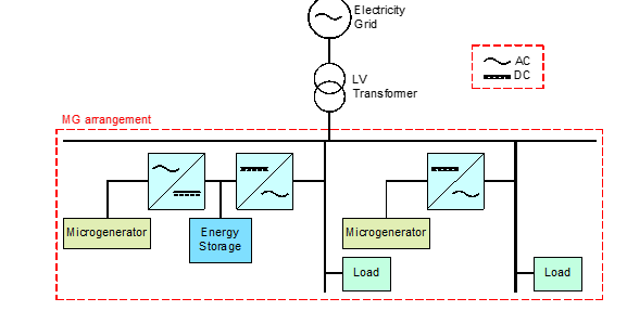
Figure 1: A simple example of MG architecture [2]

2. Comparable Works

The reduced cost of renewable energy generation combined with innovative digital technology contributes to increasing the ubiquity of smart grids, microgrids, and distributed energy generation that integrates renewable energy sources. Since 2000, the consumption of GWh has increased by 1.5 million in hydroelectric plants, 1.13 million in wind farms, and 4.44 million in solar plants. For example, in the next 20 years, renewable energy consumption will be 1.276 TWh in the European Union, 3.382 TWh in China, and 1.750 TWh in India [4].

Around the world, some MGs installations and experimental tests have been developed and updated to understand their operation in diverse topologies. While some of the studies include simply conducting research, others involve disconnecting the electric utility system. The details of very few MG projects, in the last 20 years, which have been put into action are shown in Table 1, where it is evident that the MG concept’s adaptability gives experiment settings and goals a broad range.

Table 1: Summary of a few MGs projects worldwide [5–7]

Year	Name	Location	Capacity (MW)	Supply Type
2002	DeMoTec MG	Germany	0.2	Diesel
2004	NTUA MG	Greece	0.01	Wind
2005	Aichi MG	Japan	1.2	Biogas
2008	BC Hydro	Canada	15	Diesel
2009	CERTS Lab.	USA	0.2	Gas
2012	Sevilla University	Spain	0.01	PV
2012	Juiz de Fora Lab.	Brazil	0.015	PV/Wind/Fuel cell
2013	Hawaii Hydrogen Power Park	USA	0.03	PV/Wind/Fuel cell
2014	Annobon Island	EG	5	PV
2017	Alcatraz MG	USA	0.305	PV/Diesel
2018	SPORE	Singapore	0.2	Hybrid
2019	FIE-UMSNH Lab.	Mexico	0.003	PV/Wind
2020	Agronim La Bonita	Peru	1	PV
2021	Cuenca University	Ecuador	0.329	PV/Wind/Diesel/Gas
2022	Kalbarri	Australia	5	PV/Wind

The MG approach is so versatile that has a wide range of applications in remote and off-grid communities. Radiation from the sun can be utilized as an uninterrupted resource that fits appropriately in some applications. Currently, the capacity supplied by PV energy in Ecuador is 27.65 MW, which corresponds to approximately 0.5% of the energy demand, and despite being small, it is gradually developing [8].

The National Institute of Meteorology and Hydrology of Ecuador reported that the average radiation levels were around 4.5 kWh/m² per day, in 2022, also indicating that elevated levels of around 6 kWh/m² per day were reached in some areas of the insular region and inter-Andean [8]. However, other areas such as the coast and the Amazon should not be ignored, especially the province of Guayas located in the southwest of the country, as indicated in Figure 2.

In Ecuador, PV applications have been employed in diverse sectors, such as:

• High-speed alert by small photo radars on highways.
• Water heating in Olympic swimming pools.
• Electrical supply to 370 households in the “Zero houses without electricity” project.
• Fruit drying in Manabi province is fed by PV energy.
• Institutional projects such as ESPOL rectory building where a 1.1 kW operating MG with PV/Wind source.
• The Paragachi PV plant contributes 0.998 MW to the state grid, with 4160 PV panels.
• The approved “El Aromo” PV energy project boosts Ecuador’s PV capacity almost tenfold, adding 258 MW to the current 27.65 MW [9].

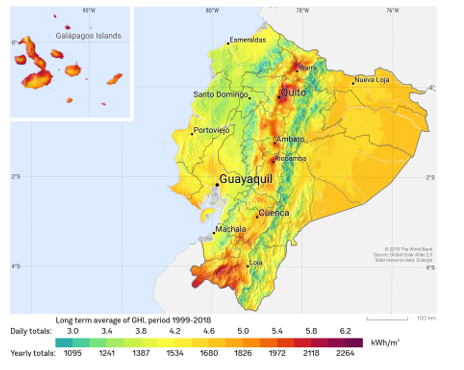
Figure 2: PV power potential in Ecuador [8]

3. Methodology

The current paper’s main topic employs a methodical and investigative approach. The area irradiance data and grid nominal electrical parameters must first be acquired to model the grid-connected system. After that, the power converters must be designed. Finally, several simulations will be run, both offline and in RT, and the results will be compared across all cascade control schemes. An MG arrangement is shown in Figure 3 which includes a PV array with a Maximum Power Point Tracking (MPPT) controller, DC-DC and DC-AC power converters, a grid-connected filter, and capacitors C_PV and C_DC for minimizing voltage ripples.

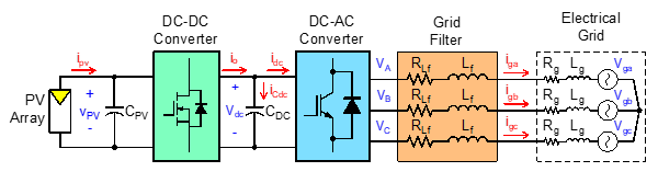
Figure 3: Complete MG sequential power circuit

3.1.  PV Panels and Arrays

PV panels, also called PV modules, are comprised of several PV cells, connected, mechanically joined, and resistant to the environmental zone to be installed. In the last years, several studies have been developed, for example in [10], where the impact of new PV panels and their estimated replacement in 10 years versus the 30 years taken as standard useful life is evaluated. That article concludes that the new panels with improved metrics such as efficiency and cost will allow competitive costs even with a 10-year replacement. Regarding PV plant location, in [11] a prediction method based on a cellular computational network to predict PV radiation for large-scale PV plants is studied. It uses geographic information to help predict radiation in neighboring areas.

A PV array made up of multiple PV panels is required to reach higher levels of PV generation. For a higher voltage, PV panels are connected in series and for a higher current they would be connected in parallel, therefore, for a higher power, a series-parallel matrix scheme would be employed. It is significant to mention that the size of PV arrays relies on the PV panels’ maximum conditions. In practice, it is standard to use photovoltaic combiner boxes to connect the output of several solar panels, hence optimizing wiring and facilitating maintenance.

3.2.  MPPT Algorithm

This algorithm is a regulation to capture the obtainable power from a PV panel during variable working conditions. This technique was implemented in the trigger circuit of the DC-DC converter to repeatedly adjust the PV array’s observed impedance and be able to keep its operation as close as possible to the maximum power point (MPP), as pointed out in Figure 4. Additionally, these characteristic curves show the MPP values, when the consumption of the PV panel is I_MPP and P_MPP at V_MPP, and the limit current/voltage values, which are the short-circuit current I_SC and the open-circuit voltage V_OC.

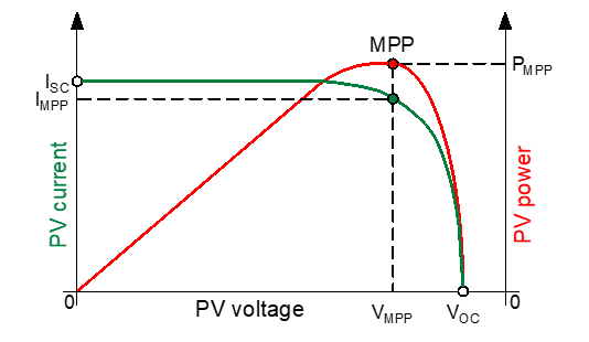
Figure 4: MPP location on Current vs. Voltage and Power vs. Voltage characteristics curves [12]

A widely accepted MPPT algorithm is the “perturb and observe” (P&O) extreme search. In an instant k, it is desired to reach the MPP, in distinction to PV array voltage/current measurements V_PV(k) and I_PV(k), and modifies its operating point slightly. Then, a comparison between this current power value P_PV(k) with the previous one P_PV(k-1) will be done, thus modifying the DC-DC converter’s duty cycle d(k) until the appropriate conditions are met [12].

Although MPPT algorithms come in various forms, according to [13], neither a deep investigation nor a comparison between various MPPT methods based on predictive control has been conducted. For this reason, in [13] this study is applied to various power converters models. It is possible to determine that the performance of the MPPT based on predictive control is related to the topology and the accuracy of the converter parameters.

The final scheme for this method is sequentially presented in the diagram shown in Figure 5, which can be employed in an algorithmic state machine (ASM), and the goal is that the duty cycle d(k) reaches a nominal value. In [12], a universal RLMPPT control method based on a reinforcement learning method is proposed, whose response adjusts the maximum power point of a PV source without any prior knowledge. Their results are close to the optimal point of the MPPT used in this article.

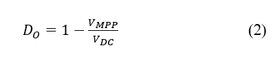
For one PV panel, the MPP data are commonly indicated in the manufacturer datasheet or its characteristic curves. This information and the MG power P_n will be helpful to determine the PV array’s size, compound by N_S panels connected in series and N_P panels in parallel as (1).

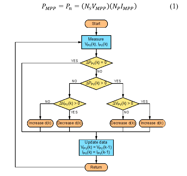
Figure 5: ASM chart of MPPT P&O algorithm [12]

3.3.  DC-DC Power Converter

These converters provide a DC voltage that can be changed between different values. The input voltage often is an unregulated DC voltage, and a DC-DC converter is used to convert it into a controlled DC output at the desired level. The operation of DC-DC converters is done with a comparison between a control voltage and a sawtooth signal v_st, oscillating at a switching frequency f_SW, and hence a period T_SW. Figure 6 shows the respective waveforms and the result of these voltages comparison, and it can be noticed that when the nominal duty cycle (D₀) increases or decreases, the switch control signal pulses shall be wider or narrower, respectively, at a constant frequency. That is the motive why this technique is called Pulse Width Modulation (PWM). It is important to mention that the control signal corresponding to D₀ will be MPPT controller output, as previously indicated in Figure 5.

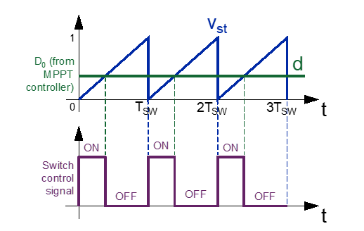
Figure 6: PWM with a comparison between sawtooth and control signals

Depending on how input/output voltage levels are related, these converters can be classified into three types: buck, boost, and buck-boost. A boost DC-DC converter, whose topology is shown in Figure 7, has been chosen to heighten the V_PV voltage into a DC link voltage v_dc capable of interfacing with the DC-AC converter.

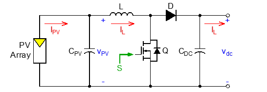
Figure 7: DC-DC boost converter power circuit fed by PV array

In this case, a MOSFET was considered as a switch because of its capacity of handling high voltage/currents. To reduce power losses, Schottky diodes should be used [14], and even these diodes have a peak current greater than typical ranges. In optimal conditions, the output V_DC voltage will be chopped according to a switch control signal S, oscillating at a switching frequency f_SW1 with a duty cycle equivalent to D₀. This desired value can be calculated as (2).

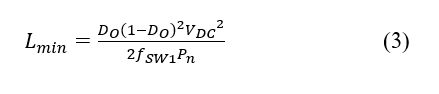
The boost converter must operate in continuous conduction mode, or when the inductor current flows continuously, therefore, a minimum value of inductance L_min shall be determined as (3), to satisfy this condition [14].

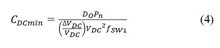
For more stable operation, an output capacitance C_DC is required. Although C_DC has a small resistance in series, it decreases the ripple in V_dc voltage, which is normally between 1% to 5%. For a given ripple percentage, the minimum capacitance C_DCmin is determined as (4), according to [14].

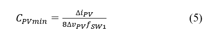
To minimize the ripple created with the PV array coupling, an input capacitance C_PV is indispensable, and its minimum value C_PVmin can be determined as (5), by [14].

3.4.  DC-AC Power Converter

The capacity to convert DC voltage into AC with the required voltage and frequency values to supply power for AC loads, either one-phase or three-phase, makes the DC-AC converter, or inverter, the most crucial component of the MG. Figure 8 illustrates a traditional two-level three-phase inverter with IGBTs for larger loads, such as those greater than 5 kW [15]. This scheme shall be implemented to maintain a balanced electrical grid. For smaller loads, the use of one-phase inverters is acceptable.

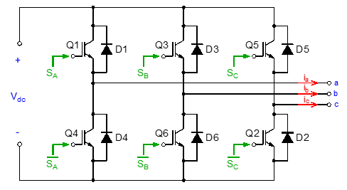
Figure 8: Two-level three-phase inverter power circuit

The IGBTs Q1, Q2, …, and Q6 are generating square outputs as expected, based on the control signals S_A, S_B, S_C, and their complements, hence using the grid filter is appropriate, which will be explained in detail in the following section 3.5. It is critical to mention that three of the IGBTs are on and the rest are off to avert short-circuits in the DC bus. In these types of converters, the SVPWM modulation scheme is commonly used because it reforms the usage of DC voltage, diminishes the generated harmonic content, and reduces switching losses.

According to (6), the switching/rotating voltage vector U_ref has three elements, one for each phase, each of which has two states: open or closed.

The U_ref vector turns counterclockwise at the inverter switching frequency f_SW, therefore, inverter behavior must adhere to the eight vectors U₀, U₁, U₂, …, and U₇. It can be demonstrated that these eight vectors, two null and six actives, have a magnitude of 2V_dc/3 and 60º phase [15], therefore six sectors will be only valid, and identified in Figure 9, where the behaviors of respective control signals S_A, S_B, and S_C are presented too.

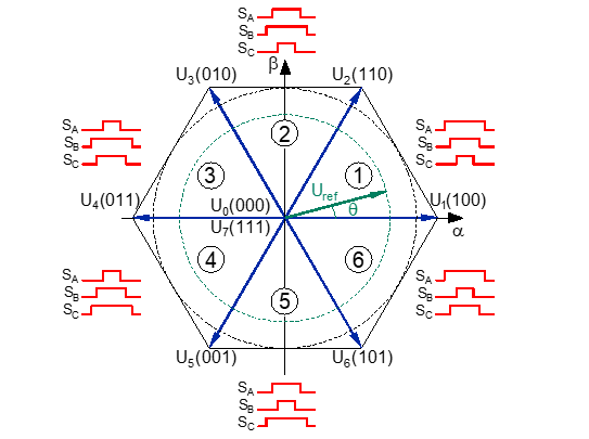
Figure 9: Space vectors for two-level three-phase inverter [15]

3.5.  Grid Filter Design

Since inverters produce harmonic content, as was already established, the quality of the energy in the electric grid will be impacted. Due to this, harmonics must be minimized, and total demand distortion must be reduced when designing a low-pass filter. The simplest option for a grid filter is an RL filter where the base inductance per phase is necessary for its calculation [16], as (7) from nominal data, in fact, the MG power P_n of the MG, the grid voltage V_n and the grid frequency f_n.

For a 10% current ripple, and considering that the value of the resistance R_Lf is 25 times greater than that of the inductance L_f, the filter components will be determined as (8) and (9):

3.6.  Control Techniques Premises in MGs

Synchronization with the electrical grid is a priority for any type of control employed in MGs, and with this, the analysis for a grid voltage vector V_ref must be turned into a linear invariant system [17] by applying the Clarke transform, to convert it from the time frame (abc frame) to an orthogonal frame (αβ frame), and then with the Park transform, to convert this vector into an orthogonal rotating frame (dq frame), as detailed in Figure 10.

Additionally, a phase-locked loop (PLL) system is required when the MG is grid-connected, which requires the electrical grid voltage V_q to distinguish the voltage phase and estimate the electrical angle that will be considered in Clarke/Park transforms. [17]. This component can be used to develop some electrical control strategies in MG inverters like:

• Voltage control, where the input voltage of the inverter is measured because this corresponds to the output line-to-line voltage.
• Active/reactive power control, where the inverter injects active/reactive power for a better MG economic operation.
• Droop control is based on voltage droop depending on active power/frequency droop increases, and reactive power decreases.

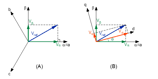
Figure 10: (A) Reference vector components in ab frame, and (B) in dq frame

The article [17] presents a description of current control methods for microgrids, especially stand-alone and inverter-based networks. In addition, the control methods are compared presenting the characteristics, control objectives, and their advantages or disadvantages. Regardless of the electrical control chosen, an electrical connection to the grid can cause disturbances, therefore, an appropriate controller must be designed.

Inverter controllers can be classified into classic and advanced. Within the classic control techniques, there is linear control, either by current or voltage, and hysteresis control, either by current or direct power, in the inverter. Furthermore, in advanced control techniques there is predictive control, either hysteresis-based, dead-band control, or model-based; intelligent control either by fuzzy logic, neural networks, or even a combination of both; and sliding mode control by voltage or current in the inverter.

4. Modeling and Control Design

4.1.  MG Mathematical Modeling

As mentioned above, the MG key component is the inverter, therefore, the DC-DC converter’s power stage will be only analyzed with the voltages and currents of interest, as shown in Figure 3. In the inverter output, the space vector voltage will be:

Applying the Clarke and Park transforms, the following rotational space vectors were obtained in the dq frame: v_s, i_s, and V_g. These vectors contain an electric component with a rotational angle ϴ_g = ω_gt = 2πf_nt, to represent these expressions in the dq frame

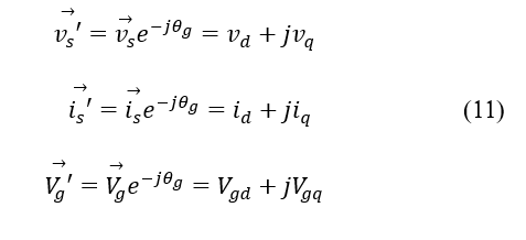
Then, the voltage space vector will be as (12) with its rotational components, and for MG dq modeling, the identity described in (13) shall be considered [18].

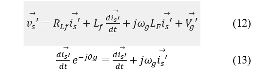
Considering a zero V_gq voltage, and based on the real and imaginary elements, the MG dynamic current models, in the dq frame, will be:

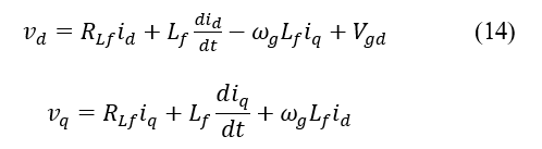
On the other hand, the relation between both the DC link power P_c, the grid power P_g and the load power P_L is considered when considering energy conservation [18], and these powers are:

4.2.  Digital Cascade Control in MGs

This control strategy is appropriate because SVPWM is frequently performed in digital signal processors, whose outputs match the pulse signals for the IGBTs [19]. These devices rely on microprocessors that run at high frequencies, which are vital in the MG field for microprocessors to contain primary and secondary control systems [20].

The cascade feedback control structure is an effective way to control electrical drives and power converters. The inner loop controllers regulate the dq currents, while the outer loop controls the main desired variable, for instance, the MG voltage, active/reactive power, or mechanical speed in AC motors. The key to the success of cascade control lies in the difference between the time constants of both loops. The response time of dq currents will be much faster.

For this control strategy works properly, some additional components must be included, such as analog to digital data converters, and vice versa, based on holding and sampling circuits. Zero-order holders (ZOH), which are utilized for voltage/current measurements and operate at a specific sampling time T_s [21], shall be included in digital cascade control schemes, as shown in Figure 11. Additionally, a digital low-pass filter (DLPF) is used to reduce DC link voltage fluctuations. There is a digital Proportional-Integral (PI) controller for the I_q with a null setpoint to give the least amount of reactive power, and the other digital PI controllers are connected in cascade to control I_d internally and V_dc externally, this being the desired variable.

For digital controllers’ tuning, in the case of I_d, the signals influenced by I_q and V_gd will be disturbances, and for I_q, the signal influenced by I_d is a disturbance. In contrast to that, for V_dc, the voltage mathematical model shall be simplified, and the voltage behavior will be stable, its component in d axis v_d will be equivalent to the MG maximum voltage, in one phase, and the DC link current i_dc will be a disturbance.

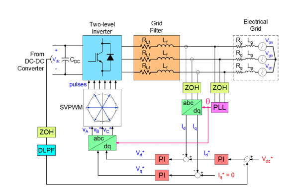
Figure 11: MG v_dc voltage regulation with digital cascade control scheme [21]

The transfer functions I_d(s)/V_d*(s) and I_q(s)/V_q*(s) will be equal and depend on the RL filter components. Then, I_d closed loop with a current controller C_i(z) will be connected in cascade with a voltage transfer function, and a voltage controller C_v(z). All these control loops are shown in Figure 12.

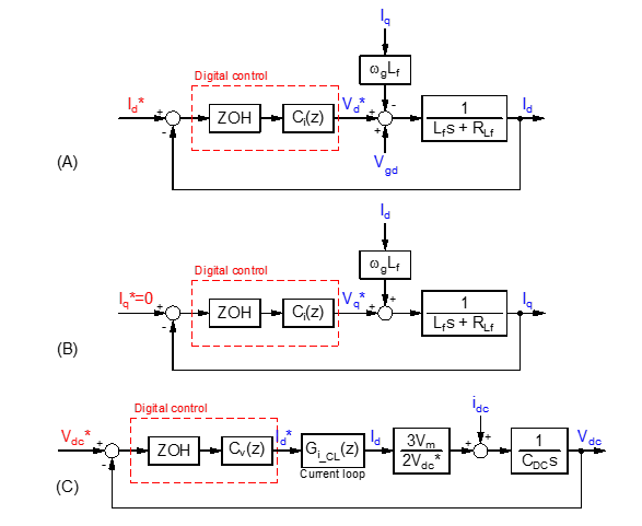
Figure 12: Block diagrams for closed-loop control systems to regulate (A) I_d, (B) I_q, and (C) V_dc

 

4.3.  Predictive Cascade Control in MGs

MBPC is model-based, good at predicting future events, and altering the current control strategy optimally, for this reason, MBPC is conducive for inverters since their model is crucial [21]. This strategy is simple and both SISO and MIMO systems can be managed. Other advantages of MBPC strategies over conventional control schemes are that they do not rely on average models, and inverter constraints like overcurrent can be considered while formulating the optimal control issue.

In MG applications, MBPC is widely used. For example, in [22], a predictive control strategy is proposed by an MG model in two layers. The first layer is responsible for optimizing power dispatch and the second layer controls diesel generation. With this method, the weights of the prediction algorithm are also manipulated. Similarly, in [23] an electrical network formed by three MGs that cooperate by sharing their power flows is modeled. Control modeling is based on predictive control, which allows cost function optimization. In that article, the power exchange occurs minimizing the generation from the micro gas turbines.

Figure 13 shows a cascade control scheme where MBPC is implemented, for dq currents regulation and an external digital PI controller for MG voltage regulation. In this case, the MBPC stage can be encapsulated as follows:

• The current prediction process depends on six cases that correspond to the combinations of the inverter’s active vectors. The objective is to decrease the errors between the reference values ​​and the present anticipated values, as described by [21].

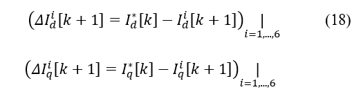
• The minimization of a dq current cost function J₁ is applied from the dq currents error, and described by [21]:

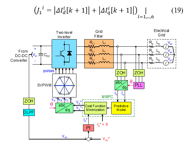
Figure 13: MG v_dc voltage regulation with combined cascade control scheme: MBPC inner loop and digital outer loop [21]

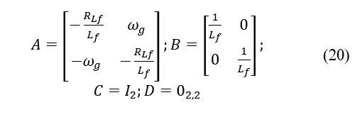
To design the MBPC controller, the dq current mathematical model, or its steady space model, must be discretized. Considering all calculated data and V_gd as a disturbance, the state matrixes indicated in (20) are obtained. Notably, this controller will manage a MIMO system with two inputs and two outputs.

Another available cascade control topology applied in MGs can be obtained by replacing the external digital PI controller with an MBPC controller. This topology provides satisfactory results but requires a lot of computational loads, which several modern hardware is capable of supplying, while a few years ago this activity was feasible but overly expensive.

Figure 14 shows a cascade control scheme where MBPC is implemented for dq currents control and MG voltage regulation. The model described by the simplified voltage transfer function detailed in Figure 12(C) was considered for designing the external MBPC controller, and the d-axis current loop was simplified as a unitary gain because the I_d* reference is reached much faster than the MG voltage.

Like the previous scheme, the MBPC stage for the outer loop can be summarized as the prediction process for v_dc voltage to decrease voltage errors, and the minimization of a voltage cost function J₂ defined by:

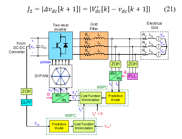
Figure 14: MG v_dc voltage regulation with MBPC cascade control scheme

5.  Simulation Results

5.1.  MG Initial Stages Design

In this paper, MG and its control were modeled and designed to feed a pumping system for agricultural irrigation in a rural area of El Triunfo, province of Guayas, which is situated in the coast region. In 2021, PV radiation had an annual mean value of 6 kWh/m² during the warmest period, in the coast area [24]. Figure 15 illustrates the trend behavior of the PV radiation in this area, and based on these data, the PV panel from the manufacturer AE SOLAR with P/N AE340SMM6-72 was chosen.

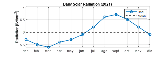
Figure 15: PV data behavior of rural zone located in El Triunfo [24]

The PV panels’ electric parameters must be chosen as a first step. These data are shown in Table 2 and were collected under standard test conditions, which are defined as being 1 kW/m² of full solar noon irradiance at a standard temperature of 25°C, for each PV panel.

By the size of the PV array, the product N_SN_P could be derived as (1) considering the MPP voltage/current values, considering that the MG power is 40 kW or the power of the PV array. In addition, N_S was chosen to be 10 because it is needed that the PV array MPP voltage shall be close to a predefined reference voltage V_dc* of 650 V, and N_P would be 12 for reaching the MPP power of the PV array. According to these predetermined values​, the PV array parameters are also indicated in Table 2.

Table 2: PV Panel and PV Array Specifications

Parameter	PV Panel	PV Array
PMPP	340 W	40.81 kW
VMPP	39.09 V	390.9 V
IMPP	8.7 A	104.4 A
VOC	46.94 V	469.4 V
ISC	9.48 A	113.76 A

For the system to be modeled, data from the subsequent stages must be determined in addition to the solar parameters. All gathered results shown in Table 3 were obtained for each indicated stage, where:

• All boost DC-DC converter components were calculated according to (2–5), with a contemplated switching frequency f_SW1 of 5 kHz.
• MPPT P&O algorithm’s maximum value will be equivalent to the calculated D₀. Other values were considered for the algorithm execution like the minimum duty cycle D_min, the initial duty cycle D_initial and the value for duty cycle increment/decrement ∆D.
• A switching frequency f_SW2 was set at 5 kHz for the inverter.
• The specifications of the Ecuadorian electrical grid, which are the grid voltage V_n of 220 V and the grid frequency f_n equal to 60 Hz, have been used to define the components of the RL filter as (8–9).
• It has been considered that the grid impedance is 10 times less than the impedance of the RL filter.

Table 3: Boost DC-DC Converter, MPPT, and Grid Filter Parameters

Parameter	Value
D0	0.3986
L	1.5227 mH
CDC	1000 mF
CPV	100 mF
Dinitial	0.01
Dmin	0
DD	±125×10–6
Lf	0.9629 mH
RLf	0.0241 Ω
Lg	0.09629 mH
Rg	0.00241 Ω

These data will be helpful for offline and RT simulations in which a 5 kW three-phase RL load with power factor FP = 0.88 will be connected after 1 s and disconnected after 2.5 s. The load connection and/or disconnection is to evaluate how well the controllers protect against disturbances while MG is operating.

5.2.  Digital Controllers Tuning

Advantageously, the discrete transfer functions for I_d and I_q are equal, and their inner dynamics depend on the RL filter calculated parameters. Therefore, for both cases, the digital PI controllers in inner loops for regulating currents will be the same. The selected gains for the I_d current controller will be essential for voltage controller tuning which depends on the inner closed loop. In the controllers’ tuning process, the best values of proportional gain K_P and integral gain K_I for dq currents and the MG voltage are shown in Table 4 with a sampling time T_s of 10 µs.

Table 4: Digital controllers’ parameters

Parameter	For Id / Iq	For Vdc
KP	0.0263	-0.0371
KI	1.9738	-0.1803

5.3.  MBPC Controllers Design

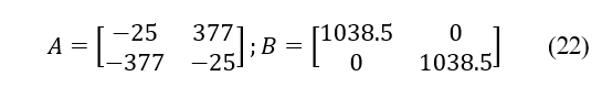
In this instance, the MBPC current controller is designed and simulated with the MATLAB mpcDesigner tool with the determined state matrixes of the dq current model, which are indicated in (22). A one-step prediction horizon N_p of 10, a one-step control horizon N_c of 2, and a sampling time T_s of 10 µs were considered.

With this sampling time, five tests were run to adjust digital PI controllers for v_dc, and the best results came from using K_P = -0.5 and K_I = -1. During this test, the shortest overshoot OS, and the fastest stabilization time T_SS were achieved. This was developed in the cascade control scheme where digital PI control is in the inner loop, and the MBPC is outer.

On the other hand, the MBPC voltage controller design for the cascade control scheme, where both loops are MBPC, was based on the simplified voltage model. Both prediction and control horizons, N_p and N_c, were the same as those used in the current control, as well as their sampling time.

5.4.  MPPT Control Performance

Before running the simulation, it is necessary to enter additional parameters to complete the compilation of the PV array block, like the number of cells per module and the temperature coefficients, and fortunately, the manufacturer’s datasheet also presents these data. In this case, the selected PV panel has 72 cells per module. Besides, the temperature coefficients α_Isc and β_Voc, determine the variation of I_SC and V_OC as a function of temperature when the PV panel operates above the standard temperature of 25°C. For the selected PV panel, the temperature coefficients α_Isc and β_Voc are 0.05%/ºC and -0.29%/ºC, respectively.

To assess the MPPT controller’s effectiveness, Figure 16 shows the PV array voltage, the output current, and the PV power delivered to the DC-DC converter. Notably, the PV array reaches the MPP because its electrical values oscillate around the MPP values listed previously, and even when the RL load is connected at t = 1s, the PV array keeps its operation around the MPP. It can be also observed that when the RL load is disconnected at t = 2.5 s, there are no induced oscillations.

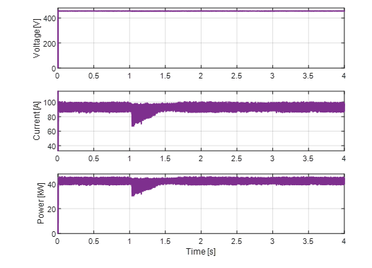
Figure 16: PV array voltage, current, and power behaviors

5.5.  Controllers Evaluation in Offline Simulations

In this section, the tests have been conducted with offline simulations, or simulations executed purely in software. To evaluate controllers, Figure 17 illustrates their performance and the behavior of MG voltage v_dc around a predefined reference V_dc* equal to 650 V with the following results:

• Initially, v_dc reaches an OS equivalent to 2.31% over the reference, with a Tss ≈ 57.1ms when digital PI control was implemented. Then, when the RL load is connected, a voltage drop of 170 V appears, and v_dc is stabilized almost equal to 0.83 s, after a dead time of 0.5 s, and when the RL load is disconnected, OS ≈ 53.97% and Tss ≈ 0.58s.
• Instead, when the inner loop was executed with MBPC and the outer loop with digital PI control, v_dc reached a higher OS ≈ 15%, with a Tss ≈ 150ms. Then, connecting the RL load, the voltage drop is less and equal to 56 V, T_SS ≈ 0.33s, and there is no presence of any dead time, and after the RL load is disconnected, OS ≈ 7.47% and Tss ≈ 0.25s.
• On the other hand, when cascade control was implemented with MBPC, v_dc reached a higher OS almost equal to 19.4%, with Tss ≈ 30.27ms. Now when the RL load is connected, the voltage drop is 22.9 V and Tss ≈ 1.29ms, without dead time too, and after the RL load is disconnected, OS ≈ 1.06% and Tss ≈ 0.52s. Unfortunately, a steady-state error (E_SS) appears when the RL load is connected, and the MG voltage could not reach the defined reference.

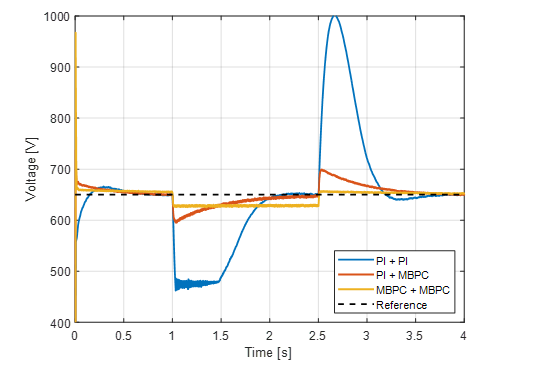
Figure 17: DC voltage behavior with both cascade controllers (Offline simulation)

Table 5 shows all the gathered ripple data present in I_d, I_q, V_d, and V_q for each cascade control scheme during the time intervals, and it is noteworthy that the control actions during MBPC are larger, four times larger for dq currents and 73 times larger for dq voltages specifically, therefore faster responses are obtained.

Table 5: DQ Currents/Voltages Ripples per Time Intervals (Offline Simulation)

PI + PI
Parameter	0 < t < 1s	1s < t < 2.5s	t > 2.5s
∆Id	16.44 A	15.71 A	16.82 A
∆Iq	15.03 A	13.13 A	13.27 A
∆Vd	0.44 V	0.43 V	0.42 V
∆Vq	0.41 V	0.39 V	0.38 V
PI + MBPC
∆Id	47.6 A	44.26 A	46.95 A
∆Iq	47.42 A	46.39 A	50.74 A
∆Vd	21.43 V	27.22 V	23.04 V
∆Vq	29.69 V	31.81 V	30.14 V
MBPC + MBPC
∆Id	38.93 A	36.63 A	40.03 A
∆Iq	48. 91 A	45.06 A	50.8 A
∆Vd	18.75 V	22.99 V	27.61 V
∆Vq	29.07 V	26.54 V	29.33 V

5.6.  Controllers Evaluation in RT Simulations

When a physical system and the CPU must operate similarly, deterministic answers must be guaranteed, and real hardware may even need to be connected in an interactive loop, RT simulation is required.

Among the advantages of verifying RT implementations, RT testing allows redefinition and verification of control systems with hardware, continuous exploration of the flexible and scalable platform, and investigation of complex, expensive, or dangerous scenarios that could be held in MGs.

The RT concept can be implemented accurately within the constraints of each system, although sampling would be different for a mechanical system compared to an electrical system. These tests are performed using the sample time T_{S_CPU}, which is the space between data processing. In this paper, it has been determined that this time is 50μs and that it is equal to all control sampling times.

 Currently, ESPOL University has the necessary equipment to conduct R&D projects in advanced industrial and academic solutions for power electronics and power systems sectors. It has the RT-LAB platform with a 32-core OPAL-RT RT simulator, fully integrated with MATLAB/Simulink, one I/O processor based on the Xilinx VC707 Virtex-7 FPGA platform, and one power amplifier OMICRON CMS 356 to exchange voltage/current signals with protection relays, or other electronic devices.

When running these RT simulations, the results tended to get even closer to V_dc*. To evaluate the same controllers, Figure 18 illustrates their performance with the following results:

• First, v_dc stabilizes so fast that there is not an OS when digital PI control was implemented. Then, when the RL load connection, a voltage drop of 58.83 V appears, and an E_SS equal to 45 V. When the RL load is disconnected, OS ≈ 30% and Tss ≈ 0.5 s.
• When the MBPC inner loop and the digital PI outer loop with, v_dc stabilizes so fast that there is not an OS. Then, connecting the RL load, the voltage drop is less and equivalent to 56.7 V, v_dc stabilized at 0.6 s, and there is no presence of any E_SS, and after the RL load is disconnected, OS ≈ 8.8% and Tss ≈ 0.23s.
• Finally, with the MBPC cascade control scheme, v_dc reached an OS ≈ 5.38%, with an Ess ≈ 19.74 V. Then, with the RL load connection, the voltage drop is 12.22 V and Ess≈ 12 V, and with the disconnection of RL load, OS ≈ 3.07% and Ess ≈ 10 V.

Similarly, to offline simulations, all gathered ripple data present in I_d, I_q, V_d, and V_q is shown in Table 6. The control actions with MBPC are larger, 3.8 times larger for dq currents and 75 times larger for dq voltages specifically.

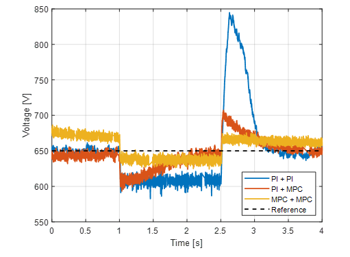
Figure 18: DC voltage behavior with both cascade controllers (RT simulation)

Table 6: DQ Currents/Voltages Ripples per Time Intervals (RT Simulation)

PI + PI
Parameter	0 < t < 1s	1s < t < 2.5s	t > 2.5s
∆Id	37.1 A	26.45 A	39.28 A
∆Iq	33.9 A	28.1 A	38.2 A
∆Vd	1.02 V	1.02 V	0.87 V
∆Vq	1.15 V	0.93 V	1.13 V
PI + MBPC
∆Id	125.7 A	115.51 A	123.41 A
∆Iq	104.4 A	103.9 A	112.8 A
∆Vd	99.31 V	93.24 V	98.64 V
∆Vq	90.6 V	91.4 V	94 V
MBPC + MBPC
∆Id	129.75 A	118.03 A	135.55 A
∆Iq	138.6 A	118 A	120.4 A
∆Vd	103.07 V	95.92 V	107.15 V
∆Vq	111.6 V	100.4 V	101.2 V

6. Conclusion and Further Results

After the performance evaluation of the MG, the correct choice of electrical components has a significant role, because the PV system’s mathematical modeling and the design premises of controllers depend on them. In the case of a component changes value, for example, the operating frequency of the electrical grid, or the V_dc* voltage setpoint, a robust control must be implemented. Even all switching frequencies shall be kept constant.

This article shows that v_dc is stabilized using various control techniques (PI + PI, PI + MBPC, and MBPC + MBPC), both in the inner loop and in the outer loop. Although v_dc is similarly stabilized using the mentioned control techniques, PI + MBPC cascade control has the best performance. Due to variations in the RL load, it was observed that the voltage spikes are acceptable compared to those that occur when using the other cascade control schemes used and do not produce steady-state voltage errors.

Offline simulations and real-times simulations are presented to validate the effectiveness of the proposed control strategies.

The studied case shows that it would be achievable to connect a 7.5 kW three-phase motor for farm irrigation. It is recommended that this load shall be a maximum of 15% of the MG-rated power.

In the case of digital control systems, it is suggested that PI controllers be used instead of PID (Proportional-Integral-Derivative) controllers, as their design is simpler and provides considerable performance. Additionally, cost savings may be realized in some cases when it is desirable to integrate hardware in the control loop.

For the MBPC design, it is a good practical idea to select an initial prediction horizon N_p and maintain it constantly while modifying other settings, such as cost function weights. N_p should not exceed 50, except when the sampling time of the controller is extremely small, and a little control horizon N_c. Thus, quadratic programming calculates fewer variables in each control interval, promoting faster current controller computations.

The MPPT algorithm with the P&O technique, and the SVPWM stage which generates the IGBT pulses, can be implemented in an FPGA. An FPGA-in-the-loop simulation can be conducted using the RT simulator. With this scenario, the use of MATLAB/Simulink for any current HDL code allows performing MG tests even with a real cascade controller.

Conflict of Interest

The authors declare no conflict of interest.

Acknowledgment

Under the auspices of the R&D Project GI-GISE-FIEC-01-2018, ESPOL Polytechnic University provided support for this research.

1. G. Elio Sanchez, S.J. Rios, “Digital Control and MBPC design for DC Voltage Regulation in a Grid-Connected PV Microgrid,” in 2021 International Conference on Electromechanical and Energy Systems (SIELMEN), IEEE: 219–224, 2021, doi:10.1109/SIELMEN53755.2021.9600409.
2. T.S. Ustun, C. Ozansoy, A. Zayegh, “Recent developments in microgrids and example cases around the world—A review,” Renewable and Sustainable Energy Reviews, 15(8), 4030–4041, 2011, doi:10.1016/j.rser.2011.07.033.
3. A. Bani-Ahmed, L. Weber, A. Nasiri, H. Hosseini, “Microgrid communications: State of the art and future trends,” 3rd International Conference on Renewable Energy Research and Applications, ICRERA 2014, 780–785, 2014, doi:10.1109/ICRERA.2014.7016491.
4. S. de Dutta, R. Prasad, “Cybersecurity for microgrid,” in International Symposium on Wireless Personal Multimedia Communications, WPMC, IEEE Computer Society, 2020, doi:10.1109/WPMC50192.2020.9309494.
5. E. Hossain, E. Kabalci, R. Bayindir, R. Perez, “Microgrid testbeds around the world: State of art,” Energy Conversion and Management, 86, 132–153, 2014, doi:10.1016/j.enconman.2014.05.012.
6. I. Latin, A. Transactions, A Review of Microgrids in Latin America: Laboratories and Test Systems, 2022.
7. Kalbarri microgrid – Australia’s largest launched, Sep. 2022.
8. INAMHI, Pronóstico del Índice Ultravioleta, Guayaquil, 2022.
9. El Aromo Solar PV Park, Ecuador, Sep. 2022.
10. J. Jean, M. Woodhouse, V. Bulović, “Accelerating Photovoltaic Market Entry with Module Replacement,” Joule, 3(11), 2824–2841, 2019, doi:10.1016/j.joule.2019.08.012.
11. I. Jayawardene, G.K. Venayagamoorthy, “Spatial predictions of solar irradiance for photovoltaic plants,” in Conference Record of the IEEE Photovoltaic Specialists Conference, Institute of Electrical and Electronics Engineers Inc.: 267–272, 2016, doi:10.1109/PVSC.2016.7749592.
12. P. Kofinas, S. Doltsinis, A.I. Dounis, G.A. Vouros, “A reinforcement learning approach for MPPT control method of photovoltaic sources,” Renewable Energy, 108, 461–473, 2017, doi:10.1016/j.renene.2017.03.008.
13. A. Lashab, D. Sera, J.M. Guerrero, L. Mathe, A. Bouzid, “Discrete Model-Predictive-Control-Based Maximum Power Point Tracking for PV Systems: Overview and Evaluation,” IEEE Transactions on Power Electronics, 33(8), 7273–7287, 2018, doi:10.1109/TPEL.2017.2764321.
14. T.K. Barui, S. Goswami, D. Mondal, “Design of Digitally Controlled DC-DC Boost Converter for the Operation in DC Microgrid,” Journal of Engineering Sciences, 7(2), E7–E13, 2020, doi:10.21272/jes.2020.7(2).e2.
15. G. Vivek, J. Biswas, “Study on hybrid SVPWM sequences for two level VSIs,” in Proceedings of the IEEE International Conference on Industrial Technology, Institute of Electrical and Electronics Engineers Inc.: 219–224, 2017, doi:10.1109/ICIT.2017.7913086.
16. H. Kim, K.H. Kim, “Filter design for grid connected PV inverters,” 2008 IEEE International Conference on Sustainable Energy Technologies, ICSET 2008, 1070–1075, 2008, doi:10.1109/ICSET.2008.4747165.
17. M.H. Andishgar, E. Gholipour, R. allah Hooshmand, An overview of control approaches of inverter-based microgrids in islanding mode of operation, Renewable and Sustainable Energy Reviews, 80, 1043–1060, 2017, doi:10.1016/j.rser.2017.05.267.
18. L. Wang, Chai Shan, Yoo Dae, Gan Lu, Ng Ki, PID and Predictive Control of Electrical Drives and Power Converters using MATLAB / Simulink, 2015.
19. S. Tahir, J. Wang, M. Baloch, G. Kaloi, “Digital Control Techniques Based on Voltage Source Inverters in Renewable Energy Applications: A Review,” Electronics, 7(2), 18, 2018, doi:10.3390/electronics7020018.
20. M. Valan Rajkumar, P.S. Manoharan, “FPGA based multilevel cascaded inverters with SVPWM algorithm for photovoltaic system,” Solar Energy, 87(1), 229–245, 2013, doi:10.1016/J.SOLENER.2012.11.003.
21. Maaoui-Ben Ikram, Mohamed Hassine, Naouar Wissem, Mrabet-Bellaaj Najiba, “Model Based Predictive Control For Three-Phase Grid Connected Converter,” Journal of Electrical Systems, 11, 463–475, 2015.
22. J. Sachs, O. Sawodny, “A Two-Stage Model Predictive Control Strategy for Economic Diesel-PV-Battery Island Microgrid Operation in Rural Areas,” IEEE Transactions on Sustainable Energy, 7(3), 903–913, 2016, doi:10.1109/TSTE.2015.2509031.
23. A. Hooshmand, H.A. Malki, J. Mohammadpour, “Power flow management of microgrid networks using model predictive control,” in Computers and Mathematics with Applications, 869–876, 2012, doi:10.1016/j.camwa.2012.01.028.
24. El clima en El Triunfo, el tiempo por mes, temperatura promedio (Ecuador) – Weather Spark, May 2022.

(Click Here)