1. Introduction

This study is an extension of our previously published [1] paper and was presented at the 7th International Conference on Data Science and Machine Learning Applications (CDMA, 2022). In this paper, we identified and detected the auditory ERP artifacts by unsuper- vised Machine Learning Algorithms (MLAs) and compared the results and features with the visual Event-Related Potential (ERP) artifacts that were presented at the CDMA conference.

Electroencephalography (EEG) is a safe and painless method of measuring the human brain’s electrical activities in real-time. In medical research, EEG experiments are very convenient. EEG measures the electric potential of the brain over a continuous time and EEG activities over a bounded time are acknowledged as Event- Related Potential (ERP) [2]. ERPs can explore the brain’s response to a specific sensory input with a high temporal resolution. In addition, ERPs are potential for the use of human biomarker, and other cerebral processes [3-5].

The oddball paradigm is one of the common experimental methods in ERP research. In the oddball paradigm, there is a sequence of monotonous stimuli, and it is irregularly interrupted by an uncommon stimulus [6]. In this study, the experimental work is comprised of a typical auditory oddball paradigm. Here, the test subject heard a series of tones with two different pitches. One of the tones is played much more frequently than other. For example, a common tone played 80% of the time with a randomly interspersed uncommon tone making up the remaining 20% of tones. It has been established by different studies that ERP gives a maximum positive peak of around 300 ms- 600 ms and the peak is higher for target/oddball stimuli compared with standard stimuli. This component is known as the P300 component [7].

However, EEG in its raw form is a mixture of neural and non-neural activities. Any non-neural activities are unnecessary in EEG research and recognized as artifacts in EEG/ERP research [8]. These artifacts may produce erroneous results in ERP studies in various ways. For example, may damage the ERP signal quality by reducing the signal-to-noise ratio , there could some arbitrary artifacts which occur infrequently for one certain condition for one test subject while for other test subjects it may occur rarely. As a result, there might be huge differences in the evaluation of two test subjects for the same experiments [9]. There are many more reasons for artifacts that may mislead the conclusion of any ERP study.

There are a huge number of sources of EEG artifacts but the most common artifacts are related to eye and body movements. In this study, our goal is to detect eye-blink artifacts, eye-movement artifacts, and body movement artifacts in normal laboratory conditions. Although much research has been done, there is no standard technique for detecting and eliminating artifacts. Addressing this, the aim of this study is to introduce a method of machine learning (ML), in which we can identify artifact corrupted ERP epochs and by removing those from the dataset, we will have a clean dataset. This experiment is done with the addition of some external effort to create artifacts. So that we could detect these artifacts. As a result, the outcomes from this study will improve the signal quality of the ERP experiment.

We applied the anomaly or outlier detection method of MLA and our data was unlabeled i.e. we applied, unsupervised MLA. Unsupervised MLAs find uncommon data points which have different properties compared to others, in any dataset. We applied three unsupervised MLAs for the detection of artifacts. They are Density-Based Spatial Clustering of Applications with Noise (DB- Scan), Isolation Forest (IsoF), and Local Outlier Factor (LOF). We measured the artifact-mixed ERP epochs detection efficiency of these methods and compared the accuracy of efficiency with the standard EEGLab method. We found the DBScan method is most efficient with 93.43% accuracy while the other methods also showed a good efficiency, ranging from 85% to 87%.

EEG is frequently utilized to analyze epilepsy, which causes variations from the norm in EEG readings. It is additionally utilized to analyze rest clutters, the profundity of anesthesia, coma, encephalopathies, and brain passing[10]. In general, EEG produces amplitude with respect to time and it is a very sensitive measurement. These measures are very important for clinical decisions. But artifacts may change or hides the information in EEG and re- moving these artifacts may take a long time for analyzing the data by extracting features. But MLAs have shown faster learning to process EEG signals [11] by outlier or anomaly detection method. Isolation Forest is an effective MLA for this detection with linear computational complexity. Screening anomaly is useful for the detection of epileptic seizures [12]. LOF can identify artifacts by producing abnormal scores using statistical methods [13]. DBScan uses a clustering-based algorithm to detect artifacts[14]. Overall, MLAs have shown effective importance in analyzing epilepsy and other neurological diseases.

The organization of the paper is as tracks: section 2 consists literature review, the experimental setup and procedure are explained in Section 3, identification of artifacts are in section 4, Section 5 contains practical implementations, and finally, results and conclusions are in Sections 6 & 7.

2. Literature Review

A lot of research has been done to remove artifacts but most methods require labeling the artifacts manually or requiring, additional hardware. For example, Electrooculography electrodes may require to place around the eyes or may necessitate data-sets containing a huge amount of data, and many more [15]. The involvement of humans to label artifacts in EEG data may be not desirable as it might be a tedious and time-consuming process [16].

In [17], the author described an unsupervised EEG artifact detection algorithm. It shows that this algorithm is effective to identify eyeblinks with 98.15% accuracy. They collected their dataset with the OpenBCI system and used EEGLab. In their experiment, sub- jects were instructed to watch a video and read articles, each for 5 minutes. They compared the methods with SVM and k-NN which are learning-based methods. But the accuracy of the performances of these methods was very low, 46.49% 67.82% comparatively.

In [18], the author established a deep learning method using Bayesian and attention modules to improve the performance of the classifier. Here, after the filtering process, to remove line noise, the artifact subspace reform (ASR) technique [19] was revised to remove an artifact that is dispersed throughout the entire scalp with a huge variance. The infomax-ICA technique was then directed to get a set of ICs establishing EEG and artifacts [20]. To end, topographic plots were grown and labeled by EEG experts. The classification accuracy was very high, around 95% but this method needs an attention module, task-dependent, and an EEG expert is required.

In [21], mthe author depicted an EEG noise-reduction scheme that customs representation knowledge to perform patient- and task- specific discovery of artifacts and correction. More specifically, their method is dependent on a given task and extracted 58 features from the signals.

3. Experimental Setup and Procedure

3.1. Dataset

This auditory oddball paradigm EEG data set is approved by the Institutional Review Board (IRB) at the University of Georgia, Athens. All of the participants provided knowledgeable permission. In this study, the number of test subjects was 13 (both male and female). They all were a minimum of 18 years of age. They had no psychiatric conditions and no hearing or eye-sight weakening. The EEG experiment had 3 setups and for every test subject, there were 3 data sets. The first data set is a mind wandering data set and the last two are artifact corrupted/test data sets. For 13 subjects, there is 13 mind wandering data sets and 26 test data sets. However, in 3 of the test data sets, almost all the ERP epochs were characterized by test subject distraction, and those 3 data sets were not considered in our study. So, there was a total of 26 test data sets.

For the recording and collection of data, an OpenBCI EEG capture system with an Ultracortex Mark IV headset was used. Here, the electrodes were connected according to the international 10-20 system along the surface of the scalp [22]. The 8-channel Cyton board was mounted to the headset. We connected electrodes to the frontal (FP1, Fz), central (Cz, C4), parietal (Pz, P7, P8), and occipital portion (O1, O2) in the human scalp (Fig. 1B). The Cyton Board was wirelessly connected via a Bluetooth (4.0 Low Energy BLE ) to a data collection computer. To generate the auditory stimuli for the ERP oddball experiments, we used a Mikromedia PIC24EP board, available from MikroElectronika Inc [23].

3.2. Data Collection Procedure

In this auditory oddball paradigm, subjects hear a sequence comprised of 2 tones with a different pitch where one of the tones is played much more frequently than the other (ex. a common tone played 80% of the time with a randomly interspersed uncommon tone making up the remaining 20% of tones).

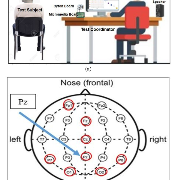
Figure 1: (A) The experimental setup of auditory oddball task. There were a series of tones with two different frequencies of 1000Hz and 2000Hz. The tones were played randomly with the stimuli duration of 200 ms and ISI of 3s 50 ms); (B) The International 10/20 system of electrode positions. The red-colored electrode positions were used to record the data in this experiment. For all the calculations, the measurements of the Pz location (marked in blue) were used.

In this experiment, to record EEG (as shown schematically in Fig. 1A), the Ultracortex Mark IV headset was used. There were 50 tones with two different pitches. One tone with 1000 Hz is known as a “ common” tone and the other with 2000 Hz, is “uncommon or oddball ”. The subject was instructed to concentrate on the uncommon tones and ignore the frequent tones. The proportion of frequent and uncommon tones was 80:20. The stimuli or tone duration was 200 ms and the Inter-stimulus Interval was 3s 50 ms.

There were 3 experimental setups. In the 1st setup, there was no instruction for the test subjects. The subject heard the tones and data were recorded. The data set from this setup is named a mind- wandering data set. At the 2nd setup, the subjects were instructed to give their special concentration to counting the uncommon/oddball tones and try to overlook the common tones. In the 3rd setup, the experimental condition was the same as in the 2nd, but we made an unexpected disturbance. For example, we made an abrupt flash on another monitor to divert the mind of the test subject, so that he/she would have somebody’s movements or blink their eyes.

The data sets collected for the last two setups are named artifact corrupted/test data sets. After completion of each dataset collection procedure, there was a 1–3-minute break of “mental rest” before initiating the next data collection interval.

3.3. Processing of Dataset

There were 3 data collection intervals for every subject and there was a total of 26 test data sets, as described in section 3.1. After recording, the data sets were protected in CSV format and EEGLab (a tool of MATLAB) was used for the primary analysis [24]. The DC offsets were uninvolved, and a band-pass filter (non-causal) of 0.1 Hz-30 Hz was used for the filtering of the EEG signals. For the ERP epochs extraction, a time window of -1000 ms to 2000 ms was bounded and ERP features were extracted in an adequate window of 200 ms to 600 ms after the commencement of the stimulus for the ERP evaluation. For further calculation, all measures (amplitude and latency) were evaluated from the uncommon stimuli at the Pz electrode position.

4. Artifacts Detection

The signal recorded in ERP experiments is a combination of EEG plus the non-neural source of activities. These non-neural sources are mainly from the induced electrical signals of the recording environment (e.g., line noise from lights and computers) and human biological activities. For example, it is very usual that while recording EEG, a test subject may blink his eye, moves his eye, he may move his head, or body, there may be muscle activities, have skin potential, and many more [25]. All of these may create non-neural signals in EEG recording and these are considered artifacts. As a result, EEG signals are often contaminated by several artifacts such as the electrooculogram (EOG), the electromyogram (EMG), electrocardiogram (ECG) and motion artifacts are a result of, for example, an eye-blink activity is an EOG artifact.

In this study, we tried to detect eye-blink, eye-movement, and body-movement artifacts. Due to the spontaneous movement of eyelids, the EOG artifact is normally always present in EEG signals. When a subject blinks his eyes, an eye-blink artifact appears as a high amplitude spike in the EEG signal [26]. Eyeblink responses are opposite in polarities compared to EEG signals and usually consist of a deflection of 50-100 V with a typical duration of 200-400 ms.

In addition, there are either horizontal eye movements or vertical ones. For a horizontal movement of eyes (HEOG), there is a higher positive voltage over the side of the head that the eyes now point toward. For a leftward eye movement, a positive-going voltage deflection is shown on the left side of the scalp, and a negative-going voltage on the right. In the case of vertical eye movements (VEOG), higher deflection shows between the electrodes below and above the eyes[27,28].

The movement of the body is very obvious for a test subject. Body movements create huge fluctuation of voltage levels and there may be high voltage levels which may shift upward or/and downward drift [29]. If these artifacts are not removed from the dataset, then the measurement or the values of the ERP features may be totally in the wrong format. All of these create huge artifacts in EEG and change the measurement levels of ERP features. Fig.2 shows the artifacts in EEG recording for subject 1.

Axis description of the figures. x-axis: time in millisecond (ms); y-axis : EEG voltage amplitudes in the microvolt

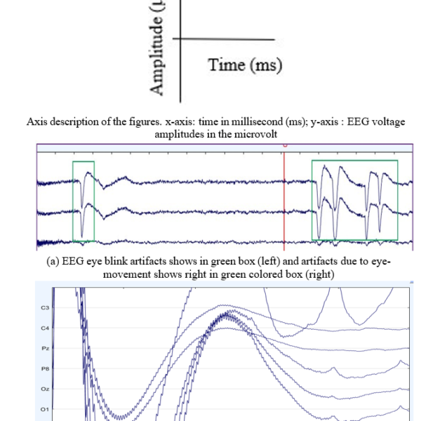
Figure 2: Examples of artifacts in EEG recordings for Subject 1

5. Practical Implementation

At first, we detected the artifact corrupted ERP epochs by a standard method (EEGLab) and after that, identified by unsuper- vised Machine Learning Algorithms (MLA). For detecting artifact corrupted ERP epochs , a maximum of 150 V (+/-) was set for peak- amplitude detection and 25 V(+/-) maximum for mean amplitude. The overall process of this study is shown in the following block diagram (Fig. 3).

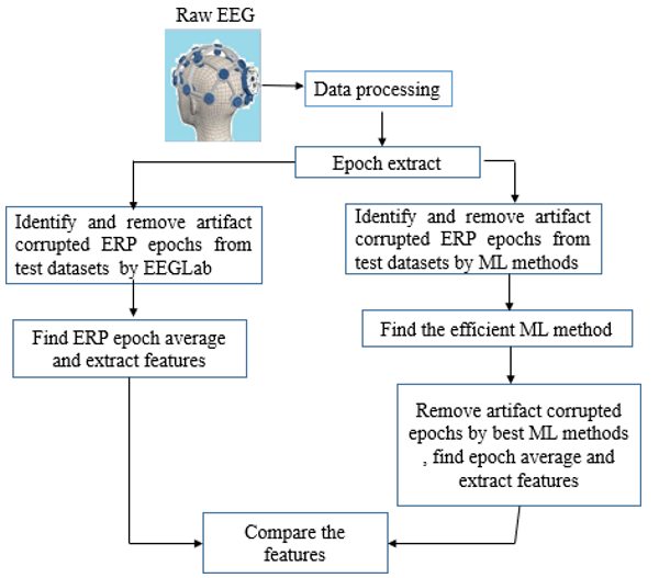
Figure 3: The block diagram of this research shows all the steps of the auditory odd- ball paradigm experiment and the comparison step with the visual oddball paradigm experiment

5.1         EEGLab: Standard method of ERP artifacts detection

EEGLab is one of the most popular EEG software for EEG analysis [30]. It is a freely available open-source toolbox [31] that provides an interactive graphical user interface (GUI), allows users to flexibly and interactively process their high-density EEG, is capable to do the dynamic brain data using independent component analysis (ICA), and able to spectral time/frequency and coherence analysis, as well as standard methods including event-related potentials (ERP) [32] and many more. For all of these reasons, we used EEGLab as a standard method of EEG/ERP analysis. Fig. 4 shows how these parameters for artifact rejection can be set for automatic artifact identification in EEGLab. Beyond these simple approaches, there are many other methods to detect and reject artifacts in the EEG data-set.

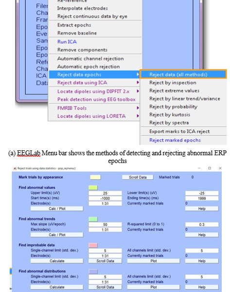
Figure 4: EEGLab processing steps for artifact corrupted ERP epochs detection

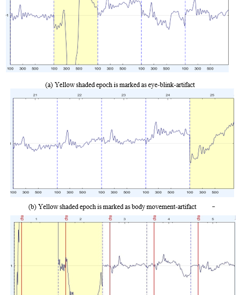
Figure 5: Examples of ERP artifacts detected by EEGLab (yellow shaded)

We performed the following steps by EEGLab [33] Toolbox:

• Filter
• Run ICA
• Remove components
• Extract epochs
• Reject Data epochs

In this study, we applied the method “Reject Data Epochs” by:

• Reject extreme values
• Reject by abnormal spectra
• Reject by the linear trend

The artifact corrupted ERPs detected by EEGLab methods, following the a bove steps are shown in Fig. 5. Among the three figures, in every figure, the yellow shaded epochs are not similar to other epochs. These are detected as anomalous ERPs by EEGLab “Reject Data Epochs” methods. For example, in fig 5A, the yellow shaded epoch ( 2nd from left) are showing a much higher peak compared to others. It is known that, for eye blink, EEG amplitudes give a higher peak. For this reason, it is marked as an eye-blink corrupted epoch.

5.1.         Machine Learning Algorithms

Machine Learning Algorithms (MLAs) generally can predict output from the given input values [34-36]. In addition, MLAs can identify the outliers in the data-set in a very fastest ode with good efficiency. Outlier points are significantly different from the majority of the other data points[37] and the process of finding the outliers in the data-set is known as anomaly detection. MLAs have both supervised and unsupervised learning approaches. Supervised learning uses labeled data to help predict outcomes. On the other hand, unsupervised learning does not use labeled  data [38]. They analyze and discover hidden patterns and return the data points with abnormal behavior. In this study, to detect the artifact corrupted ERP epochs, the following 3 features were used. i. Mean of ERP amplitude (mean), ii. The peak of ERP amplitude (peak P300), and iii. latency of the peak ERP (known as P300 ) (peak latency) in the window of 200 to 600 ms. In this study, we applied three unsupervised MLAs for identifying artifact corrupted ERP epochs based on anomaly detection. They are:

1. Isolation Forest (IsoF)
2. Local Outlier Factor (LOF)
3. DBScan

The Local Outlier Factor (LOF) algorithm is an unsupervised anomaly detection method that calculates the region density aberration of a definite data point concerning its neighbors. It considers as deviations from the norm the samples that have a noticeably lesser density compared to the neighbors[39]. In Fig. 6, there are two neighbors, C1 C2. and there are two outliers, P1, and P2. The neighbor’s numbers are a typical set of (i)more prominent than the least number of tests a cluster must contain so that other tests can be nearly exceptions relative to another cluster, and (ii) smaller than the supreme number of close-by tests and these are termed theoretically as local outliers.

Isolation Forest (IsoF) is an unsupervised MLA that separates observations by selecting random features and returns the unusual score of each test point. This algorithm describes that anomalies are data points with unusual behavior and they are few. IsoF could be a tree-based show where segments are formed by randomly selecting a feature and after that picking an arbitrary split value between the minimum and supreme worth of the chosen feature[40]. Fig. 7 shows that red circles are separated from other normal points (blue) due to unusual behavior.

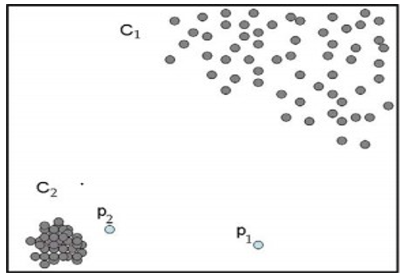
Figure 6: Local Outlier Factor. There are two neighbors, C1 C2. and there are two outliers, P1, and P2. [source: Arun Mohan,” Local Outlier Factor”, Medium.com, Dec 31, 2008]

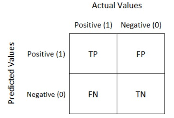
Figure 7: Isolation Forest. In this figure, red circles are separated from other normal points (blue) due to unusual behavior.

DBScan Clustering is an unsupervised MLA that’s used to gather data into clusters. It is a famous outlier detection method based on density. This process reveals central samples of high density and expands cluster density. More accurately, this algorithm sees clusters as a region of high density isolated by low density. For this relatively basic view, clusters found by DBSCAN can be in any form[41]. In this procedure, there are two sorts of parameters and three sorts of information focus. One parameter is “eps” (maximum range of the area) and another is “minpts” (least number of facts in the eps-area of a central point).

When any data point contains at least “minpts”, are known as “core points” and when the quantity of points is less than “minpts”, are known as “ border points”. In addition, within the “eps” range, when there are any points not surrounded by other points, i.e., absolutely alone in the eps range, those data point is known as an outlier, In Fig.8, there are two clusters, colored as deep-blue and green where outlier is marked as a red circle.

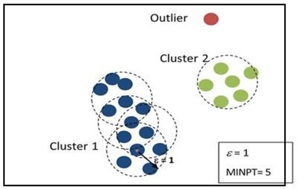
Figure 8: DBScan Cluster Technique . There are two clusters, colored as deep-blue and green where the outlier is marked as red circles. Also, eps are equal to 1 and the minimum number of points is 5.

5.2. Confusion Matrix

A confusion matrix is very useful to present the performance of any model [Fig. 9]. It consents to the visualization of the performance of the subsequent procedure. It is a table with two rows and two columns that calculates the number of true positives, true negatives, false positives, and false negatives [42]. For our calculation, we measured the accuracy (Table I) of artifact corrupted epochs for the unsupervised MLAs by the following equation:

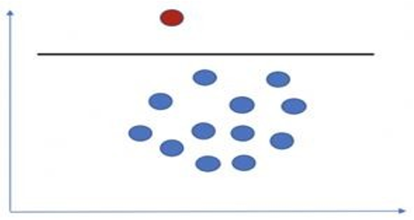
Figure 9: Confusion Matrix

α = (TP + TN)/(TP + TN + FP + FN)               (1)

In the above equation, α = Accuracy, TP = True Positive, TN = True Negative, FP = False Positive, FN = False Negative

6. Results

6.1.         Artifact corrupted Epoch Detection Accuracy

In Fig. 10, the artifact corrupted ERP epochs, detected by Isolation Forest, DBScan, and LOF methods are shown for our test subject 1. The orange colors are indicating the artifact corrupted ERP epochs.

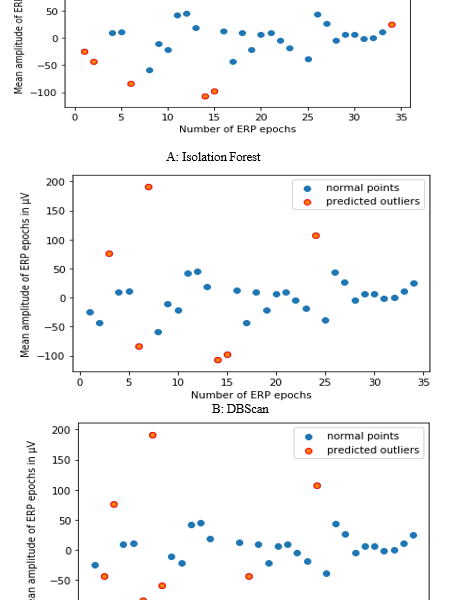
Figure 10: Three unsupervised MLAs. Here, orange circles are artifact corrupted ERP epochs and blue circles are normal ERP epochs, for the test subject 1.

Table 1: Comparison of the detection of accuracy of the arti- fact corrupted epoch (in %) with eeglab

Dataset	Isolation Forest	DBScan	LOF
D1	76	91	94
D2	88	91	88
D3	94	97	88
D4	94	91	88
D5	74	88	85
D6	94	97	97
D7	94	97	94
D8	91	97	91
D9	95	88	82
D10	94	97	94
D11	91	97	94
D12	76	94	79
D13	82	94	85
D14	91	94	88
D15	62	94	74
D16	97	94	94
D17	91	94	82
D18	91	91	82
D19	88	91	88
D20	88	97	82
D21	79	88	85
D22	82	95	84
D23	81	92	86
Average	85.54%	93.43%	87.18%

Table-I shows the detection accuracy of the artifact corrupted ERP epoch of the auditory oddball paradigm . There, artifact corrupted ERP epoch detection accuracy of three unsupervised machine learning algorithms is compared with EEGLab’s “Reject data epochs” method.

There are 23 test data-sets and named D1, D2,. . . , D23 (as described in section 3.1). Each data-set contains 50 epochs. At first, we detected the artifact corrupted epochs of the D1 data-set by EEGLab (named Data-set E1). After that, we applied 3 unsupervised MLAs ( Isolation Forest, DBScan, and LOF) to detect the outlier and named the data-sets as M1, M2 M3, respectively. Then, by confusion matrix, we compared the accuracy of M1, M2 M3 with E1 for the detection of artifact corrupted epochs. We re- peated this procedure for all the remaining 23 data-sets. All of the comparative results are shown in Table-I. All the methods showed good detection accuracy and the DBScan achieved a maximum of 93.43%. The LOF method detection accuracy was 87.18% and the Isolation Forest performed with 85.54%.

Table 2: Comparison of visual and auditory oddball paradigm artifact corrupted epoch detection accuracy

	Isolation Forest	DBScan	LOF
Audi ERP	85.34%	93.43%	87.13%
Visu ERP	79.7%	90.15%	77.95%

Table 2, shows the comparison between the auditory oddball paradigm (Audi ERP) and visual oddball paradigm (Visu ERP) for the detection of artifact corrupted ERP epochs. In our previously published paper [1], there is detail about the procedure and results of the visual oddball paradigm. The dataset is a publicly available IRB-approved dataset by the University of California, Davis. The dataset contains 30 subjects’ data. In that experiment, each subject saw five letters (A, B, C, D & E )randomly and one of these letters was assigned as a target letter, and its probability of appearance was 20%. The subject had to identify if the visual stimuli were a target or not, for every block of letters (Fig. 11). The duration of visual stimuli was 200 ms and the gap between each stimulus was 1200 – 1400 ms.

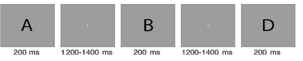
Figure 11: Visual Oddball task (Each subject saw five letters: A, B, C, D & E , randomly ,and one of these letters was assigned as a target letter, and its probability of appearance was 20%. The subject had to identify if the visual stimuli were a target or not, for every block of letters (Fig. 11). The duration of visual stimuli was 200 ms and the gap between each stimulus was 1200 – 1400 ms. );

For this visual oddball paradigm data-set, we detected three

artifacts corrupted epochs . They are artifacts due to eye blinks, due to eye-movement, and due to body movement. Both EEGLab and MLAs are applied to detect artifact corrupted epochs and compared the accuracy as we did in this study. In Fig. 12, it is shown that, for both ( visual and auditory) oddball paradigms, the DBScan per- formed with maximum accuracy while the other two methods are inconsistent with their positions.

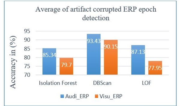
Figure 12: Comparison of artifact corrupted ERP epoch detection accuracy (on aver- age) for both auditory oddball paradigm (Audi ERP) and visual oddball paradigm (Visu ERP) ERP Signal Analysis

6.2.         ERP Parameter Analysis

At first, the mean of ERP amplitude, the peak value of ERP amplitude, and the latency of ERP peak were measured in a time window of 200ms to 600ms from the test data sets. Then we identified and removed the artifact corrupted ERP epochs (as described in Section V: A) from the test data sets. After that, we again measured the same values. After comparing the values, before and after removing the artifacts, we found a clear change in values for ERP mean and peak amplitude measures but there were no noticeable changes for the ERP peak latency measures. In Fig. 13 and Fig. 14, it is clearly shown that, for both mean and peak amplitudes, the values become lower after removing the artifact mixed epochs. For mean amplitudes it became 16.14 V from 35.4 V and, for peak amplitudes, it became 142.81 V from 223.9 V.

We also compared the values with our previously published visual oddball paradigm data set [1]. In Tables 3 & 4, values of auditory(Audi ERP) and visual(Visu ERP) ERP mean and peak amplitudes (in micro-volt ) are given. In Table 3, mean ampl is the mean amplitude before artifact corrupted ERP epochs removal and mean AR means the mean amplitude after artifact corrupted ERP epochs removal. Same meanings are applicable to Table4. From these tables and Fig. 15 Fig. 16, it is clearly shown that for both mean and, peak amplitude, the value levels were higher before the artifact corrupted ERP epochs were removed. More specifically, there are sharper differences in the auditory oddball paradigm.

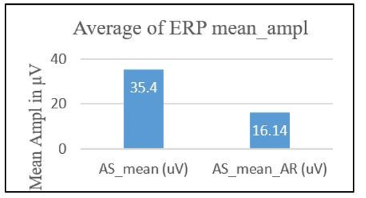
Figure 13: Comparison of the auditory mean amplitude of ERP data before and after (AR) the artifact corrupted EEG epochs are removed (uV: microvolt)

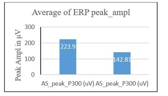
Figure 14: Comparison of the auditory peak amplitude of ERP data before and after (AR) the artifact corrupted EEG epochs are removed (uV: microvolt)

Table 3: Values of auditory and visual erp mean amplitudes in a time window of 200 to 600 ms before (mean) and after (mean ar) artifact corrupted epochs are removed

	Visu ERP	Audi ERP
mean(micro-volt)	9.28	35.4
mean AR(micro-volt)	8.59	6.14

Table 4: Values of auditory and visual erp peak amplitudes in a time window of 200 to 600 ms before (peak ampl) and after (peak ampl ar) artifact corrupted epochs are removed

	Visu ERP	Audi ERP
Peak ampl(micro-volt)	27.75	223.9
Peak ampl AR(micro-volt)	26.33	142.81

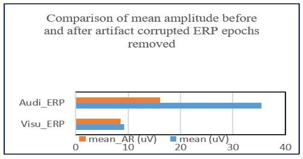
Figure 15: Comparison of the auditory ERP mean amplitude in a time window of 200 to 600 ms before and after the removal of artifact corrupted epochs (V: microvolt)

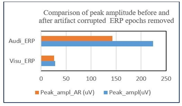
Figure 16: Comparison of the auditory ERP peak amplitude in a time window of 200 to 600 ms before and after the removal of artifact corrupted epochs (V: microvolt)

7. Conclusion

In this study, we detected ERP artifacts of the auditory odd- ball paradigm by unsupervised machine learning algorithms and compared the results with the visual oddball paradigm experiment which is our previously completed experiment. Our data were unlabeled and we found unsupervised machine learning algorithms are fairly efficient to distinguish the artifacts due to aye and body movement. Among the applied unsupervised machine-learning algorithms, the DBScan method performed with the most efficiency for distinguishing artifacts in ERPs for both audio and visual odd- ball paradigms. For the auditory ERP experiment, the accuracy is 93.43%, and for the visual ERP experiment, is 90.15%. In addition, the Isolation Forest and LOF method also showed good efficiency for the audio ERP experiment, 85.34%, and 87% respectively. On the other hand, they showed moderate efficiency for the visual ERP experiment, 79.7% and, 77.95% respectively (Table II). So, with the DBScan algorithm, we will have a cleaner ERP dataset in normal laboratory conditions with less complexity in data processing which may improve the quality of the EEG experiments.

It is very obvious that there is a huge change in amplitude levels of ERPs for the eye and body movement corrupted artifacts and normally amplitude levels lift up or down. From Tables 3 & 4, it is clear that ERP means and amplitude become lower after removing artifact corrupted epochs. In addition, there are specific differences between the audio ERP oddball paradigm experiment. On the other hand, no substantial changes were found for the peak latency, before and after artifact corrupted epoch removal.

For future research, there can be added more complexity to detect artifacts. Also, experiments can be designed to detect muscle artifacts which are one of the other common artifacts. Overall, this study may enable the use of ERPs as a strong bio-marker in EEG research in real-world experiments.

Conflict of Interest

There is not any conflict of interest.

1. R. Akhter, F.R. Beyette, “Machine Learning Algorithms for Detection of Noisy/Artifact-Corrupted Epochs of Visual Oddball Paradigm ERP Data,” in Proceedings – 2022 7th International Conference on Data Science and Machine Learning Applications, CDMA 2022, Institute of Electrical and Electronics Engineers Inc.: 169–174, 2022, doi:10.1109/CDMA54072.2022.00033.
2. S. Luck, “An Introduction to the Event-Related Potential Technique, ” Chapter 6, 2nd ed., MIT press, 2014.
3. A.K.M.A. Siddique, R. Azim, A. Islam, “Analysis of the temperature effect on the P300 component by the left and right-hand movement,” 16(1), 45–49, Oct. 2022, doi:10.9790/1676-1601014549.
4. P. Kadambi, J.A. Lovelace, F.R. Beyette, “Audio based brain computer interfacing for neurological assessment of fatigue,” in International IEEE/EMBS Conference on Neural Engineering, NER, 77–80, 2013, doi:10.1109/NER.2013.6695875.
5. M.T. Giovanetti, F.R. Beyette, “Physiological health assessment and hazard monitoring patch for firefighters,” Midwest Symposium on Circuits and Systems, 2017-August, 1168–1171, 2017, doi:10.1109/MWSCAS.2017.8053136.
6. Y.A. W de Kort L J M Schlangen Drir K C H J Smolders E Gecer, by Lotte Sap, The Influence of Light on the ERP P300 Waveform Sap, Lotte The Influence of Light on the ERP P300 Waveform THE EFFECT OF LIGHT ON THE ERP P300 WAVEFORM 1 Acknowledgement.
7. R. Akhter, K. Lawal, M.T. Rahman, S.A. Mazumder, “Classification of Common and Uncommon Tones by P300 Feature Extraction and Identification of Accurate P300 Wave by Machine Learning Algorithms,” IJACSA) International Journal of Advanced Computer Science and Applications, 11(10), 2020.
8. M.G. Asogbon, W. Samuel, X. Li, K. Dabbakuti, “Methods for removal of artifacts from EEG signal: A review You may also like A linearly extendible multi-artifact removal approach for improved upper extremity EEG-based motor imagery decoding Methods for removal of artifacts from EEG signal: A review 1,2 ShailajaKotte and,” 12093, 2020, doi:10.1088/1742-6596/1706/1/012093.
9. M.K. Islam, A. Rastegarnia, Z. Yang, “Methods for artifact detection and removal from scalp EEG: A review,” Neurophysiologie Clinique/Clinical Neurophysiology, 46(4–5), 287–305, 2016, doi:10.1016/j.neucli.2016.07.002.
10. J.A. Urigüen, B. Garcia-Zapirain, “EEG artifact removal-state-of-the-art and guidelines,” Journal of Neural Engineering, 12(3), 2015, doi:10.1088/1741-2560/12/3/031001.
11. R. Akhter, F. Ahmad, F.R. Beyette, “Automated Detection of ERP artifacts of auditory oddball paradigm by Unsupervised Machine Learning Algorithm,” in 2022 IEEE Conference on Computational Intelligence in Bioinformatics and Computational Biology, CIBCB 2022, Institute of Electrical and Electronics Engineers Inc., 2022, doi:10.1109/CIBCB55180.2022.9863055.
12. D. Steyrl, G. Krausz, K. Koschutnig, al -, L. Fiedler, M. Wöstmann, Y. Roy, H. Banville, I. Albuquerque, A. Gramfort, T.H. Falk, J. Faubert, “Deep learning-based electroencephalography analysis: a systematic review,” Journal of Neural Engineering, 16(5), 051001, 2019, doi:10.1088/1741-2552/AB260C.
13. Y. Guo, X. Jiang, L. Tao, L. Meng, C. Dai, X. Long, F. Wan, Y. Zhang, J. van Dijk, R.M. Aarts, W. Chen, C. Chen, “Epileptic Seizure Detection by Cascading Isolation Forest-Based Anomaly Screening and EasyEnsemble,” IEEE Transactions on Neural Systems and Rehabilitation Engineering, 30, 915–924, 2022, doi:10.1109/TNSRE.2022.3163503.
14. Z. Lin, F. Wen, Y. Ding, Y. Xue, “Data-Driven Coherency Identification for Generators Based on Spectral Clustering,” IEEE Transactions on Industrial Informatics, 14(3), 1275–1285, 2018, doi:10.1109/TII.2017.2757842.
15. M. Piorecký, J. Štrobl, V. Krajca, “Automatic EEG classification using density based algorithms DBSCAN and DENCLUE,” Acta Polytechnica, 59(5), 498–509, 2019, doi:10.14311/AP.2019.59.0498.
16. N. Bigdely-Shamlo, K. Kreutz-Delgado, C. Kothe, S. Makeig, “EyeCatch: data-mining over half a million EEG independent components to construct a fully-automated eye-component detector,” Annual International Conference of the IEEE Engineering in Medicine and Biology Society. IEEE Engineering in Medicine and Biology Society. Annual International Conference, 2013, 5845–5848, 2013, doi:10.1109/EMBC.2013.6610881.
17. M. Agarwal, R. Sivakumar, “Blink: A Fully Automated Unsupervised Algorithm for Eye-Blink Detection in EEG Signals,” 2019 57th Annual Allerton Conference on Communication, Control, and Computing, Allerton 2019, 1113–1121, 2019, doi:10.1109/ALLERTON.2019.8919795.
18. S.S. Lee, K. Lee, G. Kang, “EEG Artifact Removal by Bayesian Deep Learning & ICA,” in 2020 42nd Annual International Conference of the IEEE Engineering in Medicine & Biology Society (EMBC), IEEE: 932–935, 2020, doi:10.1109/EMBC44109.2020.9175785.
19. C.J.T. Kothe, “Artifact removal techniques with signal reconstruction,” Google Patents. US Patent App. 14/895,440, 2016.
20. A.K. Maddirala, K.C. Veluvolu, “Eye-blink artifact removal from single channel EEG with k-means and SSA,” Scientific Reports, 11(1), 2021, doi:10.1038/s41598-021-90437-7.
21. S. Sadiya, T. Alhanai, M.M. Ghassemi, “Artifact detection and correction in EEG data: A review,” International IEEE/EMBS Conference on Neural Engineering, NER, 2021-May, 495–498, 2021, doi:10.1109/NER49283.2021.9441341.
22. P. Schembri, M. Pelc, J. Ma, “The Effect That Auditory Distractions Have on a Visual P300 Speller While Utilizing Low-Cost Off-the-Shelf Equipment,” Computers 2020, Vol. 9, Page 68, 9(3), 68, 2020, doi:10.3390/COMPUTERS9030068.
23. LUCIO. di JASIO, “Graphics, touch, sound and usb, user interface design for embedded applications.,” 2014.
24. A. Delorme, S. Makeig, “EEGLAB: An open source toolbox for analysis of single-trial EEG dynamics including independent component analysis,” Journal of Neuroscience Methods, 134(1), 9–21, 2004, doi:10.1016/j.jneumeth.2003.10.009.
25. M. Fatourechi, A. Bashashati, R.K. Ward, G.E. Birch, “EMG and EOG artifacts in brain computer interface systems: A survey,” Clinical Neurophysiology, 118(3), 480–494, 2007, doi:10.1016/j.clinph.2006.10.019.
26. A.K. Maddirala, K.C. Veluvolu, “Eye-blink artifact removal from single channel EEG with k-means and SSA,” Scientific Reports 2021 11:1, 11(1), 1–14, 2021, doi:10.1038/s41598-021-90437-7.
27. D.W. Frank, R.B. Yee, J. Polich, “P3a from white noise,” International Journal of Psychophysiology, 85(2), 236–241, 2012, doi:10.1016/J.IJPSYCHO.2012.04.005.
28. C.J. Ochoa, J. Polich, “P300 and blink instructions,” Clinical Neurophysiology, 111(1), 93–98, 2000, doi:10.1016/S1388-2457(99)00209-6.
29. R. Martínez-Cancino, A. Delorme, D. Truong, F. Artoni, K. Kreutz-Delgado, S. Sivagnanam, K. Yoshimoto, A. Majumdar, S. Makeig, “The open EEGLAB portal Interface: High-Performance computing with EEGLAB,” NeuroImage, 224, 116778, 2021, doi:10.1016/j.neuroimage.2020.116778.
30. A. Delorme, R. Oostenveld, F. Tadel, A. Gramfort, S. Nagarajan, V. Litvak, “Editorial: From Raw MEG/EEG to Publication: How to Perform MEG/EEG Group Analysis With Free Academic Software,” Frontiers in Neuroscience, 16, 359, 2022, doi:10.3389/FNINS.2022.854471/BIBTEX.
31. C. Brunner, A. Delorme, S. Makeig, “Eeglab – an Open Source Matlab Toolbox for Electrophysiological Research,” Biomedizinische Technik. Biomedical Engineering, 58 Suppl 1, 2013, doi:10.1515/BMT-2013-4182.
32. J. Lopez-Calderon, S.J. Luck, “ERPLAB: an open-source toolbox for the analysis of event-related potentials,” Frontiers in Human Neuroscience, 8(1 APR), 2014, doi:10.3389/FNHUM.2014.00213.
33. R. Martínez-Cancino, A. Delorme, D. Truong, F. Artoni, K. Kreutz-Delgado, S. Sivagnanam, K. Yoshimoto, A. Majumdar, S. Makeig, “The open EEGLAB portal Interface: High-Performance computing with EEGLAB,” NeuroImage, 224, 2021, doi:10.1016/J.NEUROIMAGE.2020.116778.
34. T. Jiang, J.L. Gradus, A.J. Rosellini, “Supervised Machine Learning: A Brief Primer,” Behavior Therapy, 51(5), 675–687, 2020, doi:10.1016/j.beth.2020.05.002.
35. M.T. Rahman , R. Akhter, “Forecasting Stock Market Price Using Multiple Ma- chine Learning Technique, ” Preprint, 2021.
36. M.T. Rahman, R. Akhter, “Forecasting and Pattern Analysis of Dhaka Stock Market using LSTM and Prophet Algorithm,” Preprint,2021.
37. S. Sing, “Anomaly Detection Using Isolation Forest Algorithm,” Analytics Vidhya Medium, 2020.
38. M.Y. Pusadan, J.L. Buliali, R.V.H. Ginardi, “Optimum partition in flight route anomaly detection,” Indonesian Journal of Electrical Engineering and Computer Science, 14(3), 1315–1329, 2019, doi:10.11591/IJEECS.V14.I3.PP1315-1329.
39. M.M. Breunig, H.-P. Kriegel, R.T. Ng, J. Sander, “LOF: Identifying Density-Based Local Outliers,” 2000, doi:10.1145/335191.
40. A. Mavuduru, “How to perform Anomaly Detection with the Isolation Forest Algorithm, Toward Data Science, ”2021.
41. E.E.M. Schubert, “DBSCAN revisited, revisited: why and how you should (still) use DBSCAN,” ACM Transactions on Database Systems (TODS), 1–21, 2017.
42. F. Demir, “Deep autoencoder-based automated brain tumor detection from MRI data, ” Elsevier: 317–351, 2022, doi:10.1016/B978-0-323-91197-9.00013-8.

(Click Here)