1. Introduction

Advances in healthcare have made significant contributions to the longer survival and healthy lifestyle of human beings. But there are diseases that still pose a daunting challenge to the research community, Alzheimer’s Disease (AD) being an important example. AD is a major neuro degenerative  disease. The expense of Caring AD patients is quiet high. With the increase in quality of healthcare, the aging population is bound to increase and hence, we will see a greater number of people facing this disease caused by neuro degenerative changes. A treatment that follows an early detection leads to lower severity in the coming times and lowers the  risk of damage. The need for  having a Computer Aided Diagnosis system (CAD) for early and accurate AD detection and classification is  crucial. In the past years, Multi Layer Perceptrons (MLP) have been extensively used for the computer vision analysis on medical images. But the less complex Single Hidden Layer Feed Forward Neural Networks (SLFNs) have been relatively less explored. In this research work, we focus on the SLFNs, taking a step forward in realizing the potential of the ensemble ELM algorithms with the help of iterative error optimization, bagging, boosting and correlation coefficients. This work mainly focuses on evaluation of different Ensemble ELM models and comparison of performance on OASIS imaging data set. Bagging and Boosting ELM gave us good results followed by negative correlation and Incremental ELMs. We have  implemented these methods on Brain MR images unlike the different 2D data sets used in the reference implementations. As a result of the study, we intend to bring forth techniques which shall facilitate clinicians in classifying Alzheimer’s experiencing patients from normal individuals in an early stage using MRI imagery.

2. Related work

This paper is an extension of the originally submitted work in the conference  “2021 IEEE 4th International Conference on Computing, Power and Communication Technologies (GUCON). [1]

We used Modified Extreme Learning Machine algorithms to study the training computational requirements in comparison to conventional machine learning methods.[2,3] The  variations of ELMs used were, Regularized ELM (RELM) and  MLPELM [4,5].    Convolution Neural network takes more  time for training  and the desired accuracy may be difficult to achieve where as ELM is a lightweight SLFN with randomly initialized biases and weights, which when propagated onto the next layer create a Multi-Layer Perceptron without BPA (Back propagation algorithm) with ELM as the backbone of the network, and this network delivers at a faster training speed with similar accuracy rates[6].

In our implementations we had used the ELM algorithm which randomly generates the weights and biases. It tends to have a good generalizability and all the hidden layers are treated as a whole system. This way, once the feature of the previous hidden layer is extracted, the weights or parameters of the current hidden layer will be fixed and need not be fine-tuned.Therefore, this helps in getting a better accuracy and trains the network faster compared to using MLP with back propagation algorithms. It was observed that Multi Layer Perceptron had the highest accuracy while the training speed was slower, meanwhile, the RELM had lesser accuracy compared to Multi Layer Perceptron but the training speed was faster. There is a trade off between training speed and accuracy.[7,8,9]

Lot of research on new approaches with ELMs are  done. Dual-tree complex wavelet transforms (DTCWT),  Principal Component Analysis(PCA), Linear Discriminant Analysis(LDA), and ELM implementations were used to identify AD conditions. On  ADNI dataset, they could get  an  accuracy of 90%, specificity of 90% and sensitivity of 90% .[9] Another approach where Key Features Screening method based on ELMs (KFS-ELM) was implemented From  920 key functional connections screened from 4005 the accuracy is  obtained for detecting AD was 95.33% [10].

Many state-of-the art techniques like Support Vector Machine (SVM), Random Neural Network (RNN), Radial Basis Function Neural Network (RBFNN), Hopfield Neural Network (HNN), Boltzmann Machine (BM), Restricted Boltzmann Machine (RBM), Deep Belief Network (DBN), and other DL methods are compared with ELM implementations like  Circular ELM (CELM) and Bootstrap aggregated (B-ELM) and other variants. The observations are that   ELMs are faster than these techniques . Many ELM variations are being used and they are comparatively more robust. Implementation is simple and performance in terms of accuracy is also considerably better.[11,12,13]

Considering the advantages of ELMs we have incorporated the less utilized  ensemble ELMs with necessary modifications on OASIS Brain MR Data set and study the classification performance.

3. Data set

The data set is acquired from the official OASIS repository. The data set used  is OASIS-1. The data is made up of 416 subjects with their respective cross-sectional scans from 434 scan sessions. The number of T1-weighted MRI scans varies from 3 to 4 in a single-imaging session. The data acquired is restricted to right-handed individuals of both genders. The number of participants with an age above 60 with diagnosis of AD at various stages is 100.

Every imaging session was stored in its respective directory labeled with its subject ID. The subject ID format is OAS1_xxxx, where ‘xxxx’ denotes the 4digit ID of a patient(eg: OAS1_0027). All the sessions have been assigned with an ID formatted as OAS1_xxxx_MRy, here y denotes the session number of the participant (eg: OAS1_0034_MR1). A particular session is accompanied by a zip-compressed file with its respective session ID.  We have considered  totally 1412 images of which 179 Mild Demented, 145 Moderately Demented, 640 Non Demented and 448 Very Mild Demented, from the data set after Preprocessing.

4. Implementation

4.1.  Proposed Method

Our objective here is to incorporate the less explored ensemble ELMs with relevant modifications on Brain MR Data and study the classification performance on the OASIS Dataset.

The same Preprocessing steps  used in our work earlier  [1] are used for processing the images. The steps involved are initially Preprocessing, segmenting and feature extracting leading the vectors into our desired ELM classifier. The sample images and the processed images are shown below in the results section in Figure2 and Figure3. Biological implications of AD is that it  results in two distinctive abnormalities in the brain, firstly Neuro-fibrillary tangles and secondly senile plaques. A Neuro-fibrillary tangle gets originated in the cytoplasm of neurons in the entorhinal cortex, whereas the plaques found in the neocortex of the brain. Structural changes in the early stages are more dominant  in the medial temporal lobe, especially in the entorhinal cortex. With progression of the disease  both entorhinal cortex and hippocampus are the indications of the variations observed.

4.1.1. Image Preprocessing

Firstly the unrefined images are denoised and given a level of uniformity. The primary goals are echo reduction, contrast imbalance correction and image resolution rectification. A brain image is primarily comprised of Cerebrospinal Fluid(CSF), White Matter(WM) and Grey Matter(GM). The overview of the situation is that the precision with which the Regions of Interest(RoI) are ascertained among the noise created by the aforementioned features even after threshold removal of skull. We use filtering to make our classification efforts easier as it gets rid of low frequency echoes. A fixed re sizing of 256×256 and grayscale conversions are made. The finalized Preprocessing method chosen upon is median filtering which is a nonlinear method of noise elimination. It functions by iterating through each pixel and substituting each pixel with the median value of the pixels in a certain proximity range all while preserving the edges. It works on the principle of averaging and which effectively eliminates noise and blurring of sharp edges.[14]

4.1.2. Image Segmentation

The objective of this process is to segregate the image into non intersecting regions based on similarity indexes. The segmentation technique adopted here is threshold method which relies on normalizing a pixel with respect to its intensity level. It is optimal for object and background separation which comes in handy for skull removal here.[15,16]

4.1.3. Feature Extraction

It involves the recreating values by deriving them via consolidation of a large collection of data in order to bring generalization while maintaining its relevance to the task intended in future. Our focus here is texture analysis based on understanding the nature of spatial variation.  with the Gray-Level Co-occurrence Matrix (GLCM). We have used the features extracted for earlier algorithms [17]. GLCM is a square matrix representing the frequency count of appearance of a reference pixel with a particular intensity value i with respect to an adjacent neighbor pixel having an intensity value of j. Therefore, a cell (i,j) represents their cumulative occurrence count.  Their separation distance, d is also taken into account for the GLCM function computation along with regional frequency count. Further a matrix consisting of statistical values to increase the descriptive understanding is created.[18]

Our earlier implementation was of RELM and MLPELM[19,20]. Further we have worked on the performance of various Ensemble ELMs on Alzheimer’s data. Various ELMs with sigmoid  , hardlim,  gaussian and  leaky Relu functions which helps in speeding up of the training  for classification and Regression. Incremental Learning and increase in hidden nodes assist in minimizing the error. Multiclass Adaboost ELM (MAELM), Bagging Stepwise ELM and Negative Correlation ELM are suitable for  imbalanced data. They are simple, cost effective, supporting many kernels or feature mapping functions  for multi class data.Knowing ELMs require lesser time than conventional networks for training from our study performed earlier[1],  our objective here is to incorporate the above modifications to ELMs and study the classification performance on the same OASIS Dataset.We also have compared the performance of other state of art techniques like CNNs and SVM.  We have studied  different Ensemble ELMs  like ridge bagging, boosting, (Adaboost ELM )AELM and  Negative Correlation ELMs(Incremental ELM) IELM.

4.2.  Algorithms

We have implemented different ensemble ELMs and the this section will give the mathematical treatment and the methodology of implementation of these algorithms.

4.2.1. Vanilla ELM (VELM)

ELM for the SLFNs was invented in 2006.The Algorithm 1 represents the basic ELM flow. The Vanilla Extreme Learning Machine network architecture is shown in Figure 1.

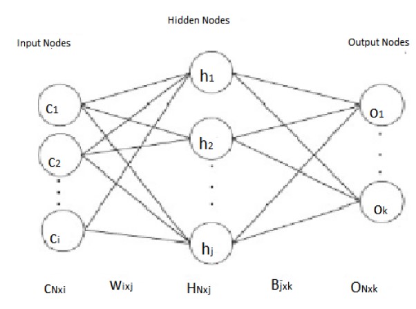
Figure 1: ELM architecture.

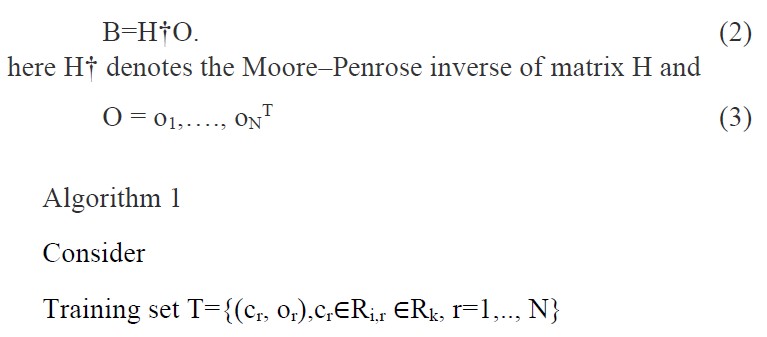
Assume N distinct samples (c_r, o_r) where c_r∈R_i and o_r∈R_k, r =1,…,N. The output hidden layer matrix H is presented as

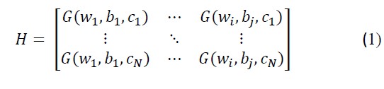
G(.) gives the  activation function, W_N×j=w₁,….,w_j represents the weight matrix between the input layer and the hidden layer and b_r represents the r^th  hidden node in a particular hidden layer bias. Both of the parameters in an particular layer are randomly initialized.[19,20]

Weights B in the output layer are to be adjusted using  the Moore–Penrose Generalized Inverse is used to compute the weights B in the between the the hidden layer and output layer

With  G• and  j representing activation function and the number of hidden nodes respectively

i: Randomly initialize desire parameters (wr,br), r =1,…..j

ii: Compute output hidden layer matrix H

iii: Successively compute matrix B

iv: Resultants are B, W and b

4.2.2. Ridge ELM

Ridrin order added to the robustness of Regularized ELM algorithm by accompanying the matrix B (output hidden layer matrix) with l₂ norm through addition to minimize the matrix B constituents by a certain degree in accordance with Bartwtt’s theory which is ‘Smaller the weights in the output layer better the generalization performance in case of feed forward neural networks.’[21,22,23] The mathematical model is

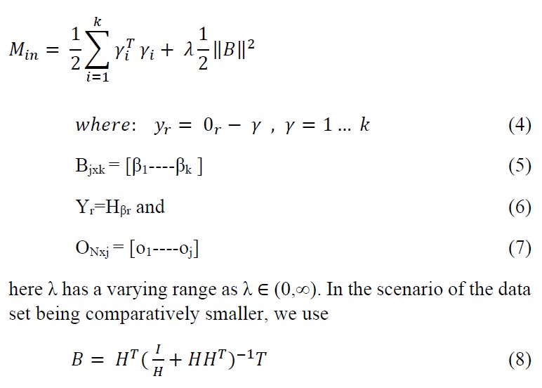
where as for the latter scenario where N ≫ j, we opt for

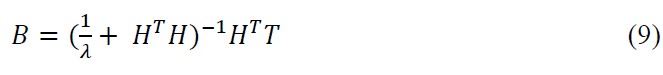
here N is the  number of training samples and  j is the   dimension of  feature space.

Algorithm 2 Consider Training set T=cr, or, cr∈Ri, or ∈Rk,  r=1,…,N

i: Randomly initialize desire parameters (wr,br), r =1,…..j

ii: Compute output hidden layer matrix H

iii: Successively compute matrix B using Eq.8 or Eq.9

iv: resultants are B, W and b

Algorithm 3 Given training set T=cr, or, cr∈Ri, or ∈Rk, r=1,…N

Learning parameter Φ and E:  number of experts

To do : Aggregation of all E experts

Loop in range  r  = 1:E

(i) By bootstrap sample in  D; get the training and validation set

(ii) train the respective expert with  Φ in training set and validation set

End : Resultants are E models of experts

4.2.3. Bagging ELM Algorithm

Bagging primarily consists of the processes of bootstrapping and aggregation. Bootstrap sampling is adopted to introduce the concept of experts generation which means the further division of training and validation set catered differently by each expert along with the putting back of samples. The models for all experts are trained with the basic algorithm for learning. Bagging uses voting for classification in order to aggregate [24,25,26].  Algorithm 3  explains this  bagging technique.[27]

4.2.4. Boosting Ridge ELM

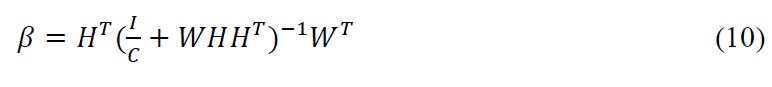
It is an ELM integrated with Boosting Ridge Regression. It consists of two initialization steps where hidden nodes are randomly initialized and the Boosting Ridge ELM chooses bias and input weights randomly. Then, a response matrix is computed for the hidden nodes. Boosting ridge then computes the output weights using boosting ridge regression. Then using feedback based on any output weights being zero, the respective hidden nodes are deleted successive to which bias and input weights matrix update is made .[28,29 ]The  algorithm is  as follows:

Algorithm 4: Given training set T=cr, or, cr∈Ri

i. Randomly initialize input weight wi and bias bi

ii. Compute hidden layer output matrix

iii. Find output weight βboosting-ridge with the help of boosting ridge regression

iv. Delete the redundant hidden node and do successive updation according to βboosting-ridge

v. Adjust the parameter values and number of iterations to get best fit

4.2.5. Negative Correlation ELM

NCELM is made up of i learners, each of which is an ELM,   c = 1. . . N, where N is the number of classifiers. The averaged output of a sample  x ∈ R

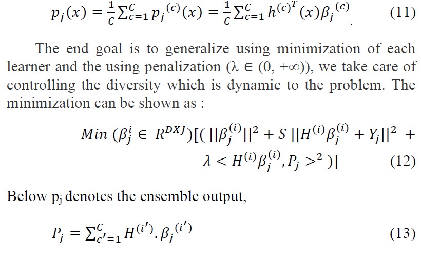
Because  appears in p_j , the proposed solution for Eq. 12 is to transform the problem in an iterated sequence, with solution of the first iteration ,(1) for c = 1, . . . , C. The output weight matrices in the r^th  iteration β (c) j,(r) ,c = 1, . . . , C, for each individual are obtained from the following optimization problem.[30]

The output weight matrices are obtained iteratively with the r^th iteration corresponding to ,(r) ,c = 1, . . . , C, shown as,

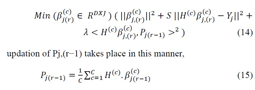
Solution can be obtained for Eqn.14 by deriving it and now by equating to 0.

Iteratively we calculate (r+1)^th term and the convergence is assured by the Banach fixed-point theorem.[30]

4.2.6. Incremental ELM

Characteristic of IELM is that the  error  decreases for every iteration and is dwindled to zero with increase in  number of hidden nodes. The trade off is between training time and accuracy as it is no more a one-shot process. The  residual error is :

E` =E−βH                                 (17)

To minimize the residual error if we are not satisfied with the minimization magnitude we restart the training of the particular node with new randomly initialized values. [31]

Algorithm 5

Given training set {(C, O)}, C is a l×N matrix which is the input of N data sets. O is a k×N matrix which is  the output of N data sets

Step 1: Set the max value J for number of nodes, initial value of residuals ε  and set current number of nodes j =0

Step 2: loop until  j < J and E >  ε : i.       Increment j by 1 ii.      Randomly initialize weight ωj and bias bj of the hidden layer neuron hj iii.    Use the activation function g(c`)  to calculate the output for the node ol c` = ωjC + bj iv.     Find the ouput vector H of  hidden  layer neurons: H = g(c` ) v.      Calculate β vi.     Re-calculate the residuals error

In the analysis 2D MRI scans were converted to 1D Numpy Arrays and then fed as input to the respective ELMs implemented.The above algorithms were implemented in Python and trained on the OASIS data set considered in our previous study as mentioned earlier. Four class classification is performed  and the comparison of the performance is discussed in the results section.

5.      Results

In our analyses using the 4 different variations of ELM and Vanilla ELM we predict the stages of the Alzheimer’s disease which were non-demented, very mildly demented, mildly demented and moderately demented as indicated in Figure2.  The various preprocessing techniques have varying effects which are visible in the Figure 3.

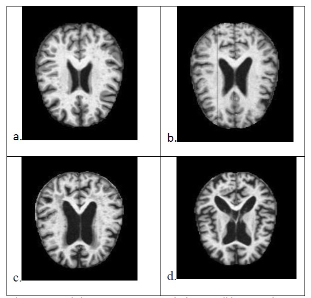
Figure 2:  Sample images, a.Non Demented ,  b.Very Mild Demented  , c.Mild Demented  , d. Moderate Demented

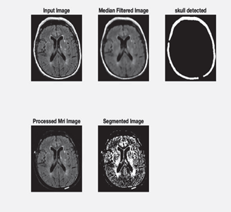
Figure 3: Sample Preprocessed images

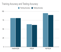
Figure 4: Accuracies of different ELMs implemented

The  results obtained for the four class classification of OASIS Data for Hardlim, RELM and MLPELM implemented in the earlier work is shown in Figure4. Timing analysis was done for which MPELM gave us good performance.

The research was focused primarily on  implementation  of algorithms  proposed by  earlier researchers and then using the appropriate quantitative initialization parameters associated with them for our Data set.

Table 1 indicates the testing accuracies obtained for  different state of art techniques implemented to compare the results with that of the ensemble ELMs.SVM and CNN-LSTM(Long Term Short Term Memory) gave us good results as indicated. With the  advantages  of ELMs , simple network and faster we find the ELMs more apt. Table 2 shows the comparison of testing accuracy for different activation functions used. Bagging and Boosting gave good results with Sigmoid and Leaky ReLU.

Table 1: Accuracies with our other implementations

Sl. No.	ELM	Testing Accuracy(%) Gaussian	Testing Accuracy (%) Sigmoid	Testing Accuracy(%) Leaky-ReLU
1	Vanilla- ELM	77.05	74.86	71.66
2	Boosting- ELM	88.42	92.32	93.47
3	Incremental- ELM	82.55	82.13	81.09
4	Bagging ELM	98.11	97.63	96%
5	Negative Correlation- ELM	83.49	87.56	84.38

Table 2: Accuracy with  other activation functions

l.No.	Model	Testing  Accuracy(%)
1	CNN	84.01
2	CNN-LSTM	98.23
3	Decision Tree	81.23
4	SVM	97.41

Table 3:  Accuracies of different implemented ELMs

Sl.No.	ELM	Training Accuracy (%) at N=50	Training Accuracy (%) at N=5000	Testing Accuracy (%) at N=5000
1	Vanilla-ELM	53.43	74.86.	72.34
2	Boosting-ELM	62.72	92.32	90.69
3	Incremental-ELM	61.63	82.13	81.23
4	Bagging ELM	63.48	97.63	97.41
5	Negative Correlation-ELM	43.00	87.56	86.03

The bagging and boosting algorithms were tried over with different activation functions which are hardlim, triangular, sigmoid, (with beta=1, used  leaky Relu to overcome vanishing gradient problem) and  gaussian . We also tuned the negative correlation coefficient in accordance with the bias and the values varied in the order of 10^-3 to 10^-4 and the best accuracy was achieved near 6×10^-3. We observed that bagging and boosting algorithms took a training time of 18-20 minutes for 5000 nodes in spite of being stepwise whereas the negative correlation ELM took 13 minutes time for training and tuning 500 nodes. The training time of negative correlation ELMs is also dependent on the designated negative correlation coefficient. The incremental ELM algorithm’s residual error value acts as a threshold value for stopping which was optimized over multiple epochs for the particular data set. Training and Testing accuracies are shown for Bagging, Boosting , Incremental and NE-ELM in the Figure 5, Figure 6 and Figure 7.

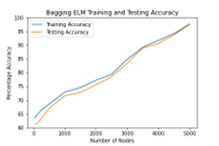
Figure 5: Accuracy of Bagging ELM

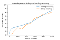
Figure 6: Accuracy of Boosting ELM

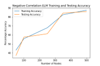
Figure 7: Accuracy of Negative-Correlation ELM

Table. 3 indicates Training and testing accuracies obtained for the algorithms implemented. Bagging gave better performance, followed by boosting and NE-ELM for 5000 nodes.

6.      Conclusion

We have implemented various ensemble ELMs like Ridge, Bagging, Boosting and Negative correlation ELMs and studied their performance on the OASIS data set. Bagging and Boosting ELM gave us good results followed by negative correlation and Incremental ELMs. These methods are implemented on Brain MR images unlike other 2D data sets used in the reference implementations.

Our approach results in better accuracy and convergence rate. The onset of impact of Alzheimer’s disease is delayed if an early diagnosis is made possible which overall helps in prevention of the incurable disease. The regularly used machine learning algorithms such as Import Vector Machine(IVM), Support Vector Machine(SVM) and Radial Basis Functions require iterative training by adjustment of parameters to reduce the error. They are time-intensive and require manual assistance for obtaining the desired accuracy. In our proposed method, we have used the ELM algorithms which rely entirely on random initialization which creates a generalized inductive bias, thus obviating the need for fine-tuning for each layer or node addition.

7.      Future scope

The research on Ensemble ELM networks can be taken forward with the infusion of deep learning kernels such as Convolution ELMs and RNN-ELMs which promise the successful results of dense multi-layered networks without the time indulgence put into fine tuning. If algorithms like RNN-ELM which make use of temporal space weights are used along with Dual-Tree Complex Wavelet Transform (DTCWT) we stand to gain great benefits from the directional sensitivity subsiding shift in variance. It can be implemented and tested on PET (Positron Emission Tomography) Data. Can further work on  improving on  timing constraints [1]. The time required for execution can be optimized.

Conflict of Interest

The authors declare no conflict of interest.

Acknowledgments

Data set is from OASIS – OASIS-1: Cross-Sectional: Principal Investigators: D. Marcus, R, Buckner, J, Csernansky J. Morris

1. A. Hari, V. Rajanna, V. A, R. Jain, “An Extreme Learning Machine based Approach to Detect the Alzheimer’s Disease,” 1–6, 2021, doi:10.1109/GUCON50781.2021.9573589.
2. R.K. Lama, J. Gwak, J.-S. Park, S.-W. Lee, “Diagnosis of Alzheimer’s Disease Based on Structural MRI Images Using a Regularized Extreme Learning Machine and PCA Features,” Journal of Healthcare Engineering, 2017, 5485080, 2017, doi:10.1155/2017/5485080.
3. K.A. Johnson, N.C. Fox, R.A. Sperling, W.E. Klunk, “Brain imaging in Alzheimer disease,” Cold Spring Harb. Perspect. Med., 2(4), a006213, 2012.
4. R.N. and G.A. Palimkar Prajyot and Shaw, “Machine Learning Technique to Prognosis Diabetes Disease: Random Forest Classifier Approach,” in: Bianchini Monica and Piuri, V. and D. S. and S. R. N., ed., in Advanced Computing and Intelligent Technologies, Springer Singapore, Singapore: 219–244, 2022.
5. X. Liu, L. Wang, G.-B. Huang, J. Zhang, J. Yin, “Multiple kernel extreme learning machine,” Neurocomputing, 149, 253–264, 2015, doi:https://doi.org/10.1016/j.neucom.2013.09.072.
6. S. Mandal, V.E. Balas, R.N. Shaw, A. Ghosh, “Prediction Analysis of Idiopathic Pulmonary Fibrosis Progression from OSIC Dataset,” in 2020 IEEE International Conference on Computing, Power and Communication Technologies (GUCON), 861–865, 2020, doi:10.1109/GUCON48875.2020.9231239.
7. G. Huang, G.-B. Huang, S. Song, K. You, “Trends in Extreme Learning Machines: A Review,” Neural Networks, 61, 2014, doi:10.1016/j.neunet.2014.10.001.
8. S. Suhas, C.R. Venugopal, “MRI image preprocessing and noise removal technique using linear and nonlinear filters,” in 2017 International Conference on Electrical, Electronics, Communication, Computer, and Optimization Techniques (ICEECCOT), 1–4, 2017, doi: 10.1109/ICEECCOT.2017.8284595.
9. D. Jha, S. Alam, G.-R. Kwon, “Alzheimer’s Disease Detection Using Extreme Learning Machine, Complex Dual Tree Wavelet Principal Coefficients and Linear Discriminant Analysis,” Journal of Medical Imaging and Health Informatics, 8, 881-890(10), 2018.
10. J. Lu, W. Zeng, L. Zhang, Y. Shi, “A Novel Key Features Screening Method Based on Extreme Learning Machine for Alzheimer’s Disease Study,” Front Aging Neurosci, 14, 888575, 2022.
11. J. Wang, S. Lu, S.-H. Wang, Y.-D. Zhang, “A review on extreme learning machine,” Multimedia Tools and Applications, 81(29), 41611–41660, 2022, doi:10.1007/s11042-021-11007-7.
12. S. Grueso, R. Viejo-Sobera, “Machine learning methods for predicting progression from mild cognitive impairment to Alzheimer’s disease dementia: a systematic review,” Alzheimer’s Research & Therapy, 13(1), 162, 2021, doi:10.1186/s13195-021-00900-w.
13. M. Odusami, R. Maskeliunas, R. Damaseviv cius, T. Krilavicius, “Analysis of Features of Alzheimer’s Disease: Detection of Early Stage from Functional Brain Changes in Magnetic Resonance Images Using a Finetuned ResNet18 Network,” Diagnostics (Basel), 11(6), 2021.
14. S. Leandrou, S. Petroudi, P.A. Kyriacou, C.C. Reyes-Aldasoro, C.S. Pattichis, “Quantitative MRI Brain Studies in Mild Cognitive Impairment and Alzheimer’s Disease: A Methodological Review,” IEEE Rev Biomed Eng, 11, 97–111, 2018.
15. G.V.S. Kumar, V.K. .R, “REVIEW ON IMAGE SEGMENTATION TECHNIQUES,” International Journal of Scientific Research Engineering & Technology (IJSRET), 3, 992–997, 2014.
16. M. Al-amri, D. Kalyankar, D. S.D, “Image segmentation by using edge detection,” International Journal on Computer Science and Engineering, 2, 2010.
17. D. Tian, “A review on image feature extraction and representation techniques,” International Journal of Multimedia and Ubiquitous Engineering, 8, 385–395, 2013.
18. T. and S.R.N. and G.A. Sinha Trisha and Chowdhury, “Analysis and Prediction of COVID-19 Confirmed Cases Using Deep Learning Models: A Comparative Study,” in: Bianchini Monica and Piuri, V. and D. S. and S. R. N., ed., in Advanced Computing and Intelligent Technologies, Springer Singapore, Singapore: 207–218, 2022.
19. W. Deng, Q. Zheng, L. Chen, “Regularized Extreme Learning Machine,” in 2009 IEEE Symposium on Computational Intelligence and Data Mining, 389–395, 2009, doi:10.1109/CIDM.2009.4938676.
20. J. Tang, C. Deng, G.-B. Huang, “Extreme Learning Machine for Multilayer Perceptron,” IEEE Transactions on Neural Networks and Learning Systems, 27(4), 809–821, 2016, doi:10.1109/TNNLS.2015.2424995.
21. R. Yangjun, S. Xiaoguang, S. Huyuan, S. Lijuan, W. Xin, “Boosting ridge extreme learning machine,” in 2012 IEEE Symposium on Robotics and Applications (ISRA), 881–884, 2012, doi:10.1109/ISRA.2012.6219332.
22. B. Jin, Z. Jing, H. Zhao, “Incremental and Decremental Extreme Learning Machine Based on Generalized Inverse,” IEEE Access, 5, 20852–20865, 2017, doi:10.1109/ACCESS.2017.2758645.
23. G. Feng, G.-B. Huang, Q. Lin, R. Gay, “Error Minimized Extreme Learning Machine With Growth of Hidden Nodes and Incremental Learning,” IEEE Transactions on Neural Networks, 20(8), 1352–1357, 2009, doi:10.1109/TNN.2009.2024147.
24. Z.X. Chen, H.Y. Zhu, Y.G. Wang, “A modified extreme learning machine with sigmoidal activation functions,” Neural Computing and Applications, 22(3), 541–550, 2013, doi:10.1007/s00521-012-0860-2.
25. C. Perales-González, “Global convergence of Negative Correlation Extreme Learning Machine,” Neural Processing Letters, 53(3), 2067–2080, 2021, doi:10.1007/s11063-021-10492-z.
26. P. Khan, Md.F. Kader, S.M.R. Islam, A.B. Rahman, Md.S. Kamal, M.U. Toha, K.-S. Kwak, “Machine Learning and Deep Learning Approaches for Brain Disease Diagnosis: Principles and Recent Advances,” IEEE Access, 9, 37622–37655, 2021, doi:10.1109/ACCESS.2021.3062484.
27. M. Yang, J. Zhang, H. Lu, J. Jin, “Regularized ELM bagging model for Tropical Cyclone Tracks prediction in South China Sea,” Cognitive Systems Research, 65, 50–59, 2021, doi:https://doi.org/10.1016/j.cogsys.2020.09.005.
28. A.O.M. Abuassba, D. Zhang, X. Luo, A. Shaheryar, H. Ali, “Improving Classification Performance through an Advanced Ensemble Based Heterogeneous Extreme Learning Machines,” Computational Intelligence and Neuroscience, 2017, 3405463, 2017, doi:10.1155/2017/3405463.
29. Y. Jiang, Y. Shen, Y. Liu, W. Liu, “Multiclass AdaBoost ELM and Its Application in LBP Based Face Recognition,” Mathematical Problems in Engineering, 2015, 1–9, 2015, doi:10.1155/2015/918105.
30. S. Wang, H. Chen, X. Yao, “Negative correlation learning for classification ensembles,” in The 2010 International Joint Conference on Neural Networks (IJCNN), 1–8, 2010, doi:10.1109/IJCNN.2010.5596702.
31. S. Song, M. Wang, Y. Lin, “An improved algorithm for incremental extreme learning machine,” Systems Science & Control Engineering, 8(1), 308–317, 2020, doi:10.1080/21642583.2020.1759156.

(Click Here)