1. Introduction and Related works

This paper is an extension of the work originally presented in IEEE System on Chip Conference 2017 [1]. This extension contains a more detailed explanation of the applied system level synthesis method. An additional practical benchmark is also solved and evaluated.

The system-level synthesis procedure of high-performance multiprocessor systems usually starts by some kind of a task description regarding the requirements and their desired priorities. The task description is usually formalized by a dataflow-like graph or by a high level programming language [2] [3]. To each component processor of the multiprocessor system, a subtask is assigned basically by intuition considering various special requirements (communication cost, speed, pipelining, etc.). The definition of the subtasks, i.e. the decomposition of the task strongly influences the cost and performance of the whole multiprocessing system. Therefore, comparing and evaluating the effects of different task decompositions performed by applying systematic algorithms may help the designer to approach the optimal decisions in the system-level synthesis phase [4]. Our proposed method can also be considered a design space exploration as shown in [3-5]. In [5] the hardware-software partitioning problem is analyzed and various solutions are compared and evaluated. This approach refers formally only to special two-segment decompositions. These can be extended for multi-segment cases by utilizing several high performance heuristic algorithms [6], [7]. However, in case of such extensions for multiprocessing architectures [8], the decomposition algorithm and the calculation to find beneficial communication cost and time become rather complex and cumbersome. Other special aspects of multi-segment partitioning problems can be found in [9] at the synthesis of low-cost system-on-chip microcontrollers consisting of many integrated hardware modules. For avoiding to the aforementioned difficulties, the paper presents a novel method called DECHLS based on combining decomposition and modified high level synthesis algorithms.

This paper is organized as follows. Section 2 contains the overview of the proposed novel system-level synthesis method (DECHLS). The decomposition algorithms applied in the experimental DECHLS tool and the applied performance metrics are presented in Section 3. The embedded multiprocessing systems to be redesigned by the experimental DECHLS tool, the redesigned variations obtained by DECHLS and the evaluation of the results are presented in Section 4. The conclusion is summarized in Section 5.

2. Overview of the System-Level Synthesis method DECHLS

Our method (DECHLS [1]) is based on combining decomposition (DEC) with high level synthesis (HLS) algorithms. One of the main steps in HLS tools [10], [11] is the allocation executed after scheduling the elementary operations. The aim of scheduling is to determine a beneficial start time for each elementary operation to attempt allocating them optimally into processing units [12]. Usual optimality criterions in HLS tools are the minimal number of processing units, the lowest cost and the highest speed in pipelining [10], [11], or the lowest power consumption [12]. The elementary operations allocated into the same processing units compose the subtasks. However, such subtasks provided by the HLS tools are strongly determined by the usual scheduling algorithms and so, not enough freedom is left for satisfying special multiprocessing requirements in further synthesis steps. Instead of modifying and extending the usual HLS scheduling algorithms [13-16] for fulfilling these special requirements, our DECHLS method attempts to satisfy these on a higher priority level by executing the decomposition into subtasks already before the HLS phase. A similar approach is presented in [17] called clustering. In [17] the power efficiency is attempted to be optimized by clustering in pipeline systems at a given throughput. The resulting structure can be considered a special decomposition that may decrease communication and hardware costs as well, but these benefits are not analyzed directly. Our preliminary decomposition can be considered a kind of a preallocation providing more freedom to fulfill special multiprocessing requirements. Based on the subtasks (called segments hereinafter) obtained by decomposition, a segment graph (SG) can be constructed. The SG can serve as an elementary operation graph (EOG) of the modified HLS tool. Thus, the scheduling and allocation algorithms in the modified HLS tool refer to the component processors in further steps. In this way, the decomposition executed before the HLS steps can influence the result on a higher priority level. Thus, DECHLS is based on combining the decomposition (DEC) and modified high level synthesis (HLS) algorithms. The main contribution of the DECHLS is that these two steps are integrated into the same design tool enabling the designer to generate, evaluate and compare various alternative results. The list of user-defined requirements, required inputs and outputs of the DECHLS process is outlined in Fig.1. The workflow of the DECHLS method is shown in Fig 2.

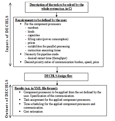Figure 1. Inputs and outputs of the DECHLS method

There is also a possibility in DECHLS method to generate the EOG for the HLS tool immediately from the task description without preliminary decomposition. If decomposition is intended to be made, then the desired number of segments can either be prescribed or calculated by the decomposition algorithm. In both cases, the modified HLS tool receives the segment graph (SG) as EOG. If the user decision is that pipeline mode is not required, then the process of DECHLS is finished and the allocated nodes formed from the segment graph (SG) define the tasks for the component processors. If however, the pipeline mode is desired, then the applicable value of the pipeline initialization interval called further on restart time (R) is calculated. Most of the HLS tools [10], [11] can attempt to ensure a user-defined desired restart time (Rd.). If R≤Rd, is not the case, then the HLS tool [10] applied in the experimental DECHLS version reduces R by buffer insertion and/or by applying multiple copies of nodes. If the cost of the resulting multiprocessing system is not acceptable, then allowing a longer latency time L (the longest time of processing an input data in the allocated segment graph) in pipeline mode may reduce the cost by calculating a new schedule [18]. The user can increase L in more iteration steps and the value of dL is also definable by the user. If the cost is acceptable, then the process of DECHLS is finished.

The scheduler applied in the experimental DECHLS version is a modified force-directed one [19]. Results of the usual force-directed schedulers strongly depend on the order of fixing the operations within their mobility domain (i.e. between the earliest and latest possible start time) [20]. In contrary, our modified scheduler generates a list of all operations according to the length of their mobility and the operations having the shortest mobility are fixed first (i.e. the top of the mobility list). After fixing an operation, the mobility list is recalculated and a next operation is chosen, and so on until each operation has been fixed.

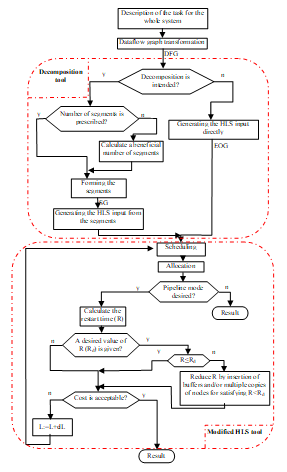Figure 2. Design flow of the DECHLS method

Increasing the latency (L) can be simply implemented in any HLS tool. The simplest way is to introduce an extra fictive operation parallel with the original operation graph. The execution time of this extra operation is assumed to be equal to the desired latency value. This extra operation receives all inputs of the original operation graph, and its output enables all outputs of the original graph. This extra operation could be added only before scheduling, and it must be removed before allocation, since it is not an operation to be executed by the resulting system.

3. Decomposition of the Task Description

The decomposition step of the DECHLS method starts from a dataflow-like task description (DFG). The nodes of this graph represent inseparable operations, and the edges symbolize data dependencies between the operations. The decomposition algorithm should define disjoint segments containing each of them several (at least one) operations. The segments represent subtasks of the task description and form a segment graph (SG) that may be the input of the HLS part in the DECHLS system. The edges in SG represent data communication between segments, edges are weighted by the communication burden. The nodes in SG representing the subtasks are also weighted by the longest execution time of the subtask. The execution time of a segment is the sum of execution times of the elementary operations assigned into this segment. The reason of this is that the processors are assumed to execute serially all elementary operations to be assigned to them. For comparing and evaluating the effect of different task decompositions, the desired number of segments is user-definable. The distribution of workload between segments is arranged beneficially for pipeline implementation (i.e. as far as possible equally) and at the same time, the communication load (edge weights) between the segments should also be kept possibly low. Beside these aims, the decomposition algorithm must not produce segment cycles as shown in Fig. 3 and [21]. Such cycles may cause deadlocks and it is difficult to handle them in pipeline mode. Handling or eliminating the cycles depends on the HLS tool applied in DECHLS system [10] [11]. The decomposition algorithms may produce cycles in the SG, even if the task description (EOG) is acyclic. Therefore, only such decomposition algorithms are allowed in DECHLS system, which guarantee cycle-free SG-s [21]. In our experimental DECHLS tool, this difficulty is avoided by generating the allowable edge cutting places before starting the decomposition algorithm [21].

The decomposition algorithms may yield segments consisting of extremely different number of elementary operations. In the further steps, the allocation algorithm in DECHLS may provide processors with extremely different workload.

Therefore, the user has to decide, whether applying always the just fitting processors or choosing equally suitable identical processors. A very simple cost calculation and comparison (i.e. the number of processors) can be applied in the latter case. Therefore, identical processors are assumed in the further discussions and in the solutions of the practical examples.

A set of decomposition algorithms is available in [21-23]. Two of them seemed to be the most suitable for DECHLS: the spectral clustering (SC) and the multilevel Kernighan–Lin (KL) method. The spectral clustering is applied for the illustrative redesigning examples in two versions: the number of segments is prescribed or it is calculated by the algorithm. These decomposition algorithms are suitable to illustrate the DECHLS method and yield acceptable results. However, other more advanced or flexible decomposition methods like [25] or [26] could also be applied in DECHLS.

For comparing and evaluating the solutions obtained by DECHLS, some performance metrics could be assumed. These metrics are flexibly definable and extendable by the user. The experimental metric criteria applied in Section 4 for comparing the results are as follows. The hardware cost is calculated simply as the number of processors, assuming that each processor has the same performance specification.

– The pipeline restart time versus the hardware cost is plotted for helping the beneficial and economical choices and forecasting the consequences.

– The longer latency in pipeline mode [18] [29] may reduce the hardware cost without significant effects on the restart time.

Figure 3. Allowable (b) and not allowable (a) decomposition [19]

4. Benchmark Solutions and Evaluations

4.1.  A sound source localization system

A sound source localization system is presented in [27] as a relatively simple multiprocessing system. The segment graph (SG) constructed probably by intuition is shown in Fig. 4.

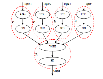Figure 4. Intuitively decomposed and allocated segment graph (SG)  (sound source localisation) [27]

The task to be solved is decomposed into 10 subtasks (each of them is a separate segment) FFT1, … FFT4, SC1, … SC4, VOTE, HT as shown in Fig. 4. The segment functions are as follows. FFTs execute a 512 point real fast Fourier-transformation. SCs perform noise power estimation for each channel of input data. VOTE detects whether a detectable sound was present on at least two channels in the current sample, and the noise is sufficiently low at the same time. The longest segment is HT that performs the hypothesis testing method [27] for determining the source coordinates of the sound.

The implementation in [27] is based on five processors (P1, … P5) as shown in Fig. 4. One of the consequences of this intuitive solution is that P5 has the computationally most expensive subtask requiring approximately 5 times faster processor than the other ones. Therefore, the speed of the whole system strongly depends on the implementation of P5.

In order to evaluate new decompositions, the given segment graph has to be expanded into an elementary operation graph (EOG), the nodes of which are considered atomic inseparable elementary operations. A possible method may start with a high level language description of the segments in SG. Each segment may correspond to a function in the high level language description. This function may call other functions and so on until getting functions considered inseparable.

For the sake of simplicity, software loops in the task description can also be considered single inseparable nodes, because the complex loop handling would be an additional difficulty (e.g. in pipeline systems [28]). This simplification does not affect the essence of the further steps.

The transformation process from SG to EOG is illustrated by a simple example in Fig. 5.

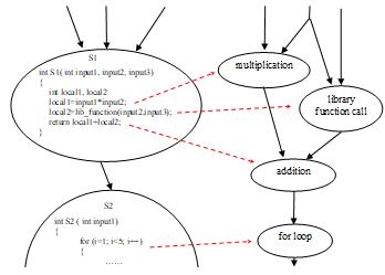Figure 5. Expanding a SG into an EOG (the small program fragments in segments are only to illustrate the process)

From the SG in Fig. 4, this transformation yields an EOG with over 160 nodes.

For further handling of the EOG, execution times should be assigned to each elementary operation. For these assignments, the specifications of processors to be applied should be known. In the original implementation [27], two different processor types have been used: the slower MSP430 and the faster ARM7. The faster ARM7 processor has been chosen probably because of the large memory demand of HT. The slower and cheaper processors, (16 bit MSP430 microcontrollers) have been found suitable for the remaining tasks.

Further on, the execution times will be expressed by the number of time steps as used in our modified HLS tool [10]. In this way, the calculation becomes independent from the clock speed. All time data, including data of the existing systems will also be expressed in time steps for comparison.

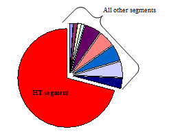Figure 6. The relative execution time proportions of the segments in Fig. 4.

Fig. 6 shows the relative execution time values of the segments determined according to the intuitive decomposition shown in Fig. 4. Note, that this solution yielded great differences in the execution times of the processors that may cause unnecessary constraints in case of pipelining.

The comparative solutions obtained by applying DECHLS approach to a uniform workload distribution between the processors.

4.2.  Evaluation of the existing decomposition for the sound source localization

As it has been mentioned earlier, only identical processors are assumed in both redesign examples. In order to achieve the best results with identical processors, all the segments require approximately identical execution times. To illustrate the problem, our modified HLS tool provides the plot in Fig. 7. calculated from the intuitive SG in Fig. 4. The execution times are calculated assuming that only MSP430 microprocessors are applied in the implementation. Such an implementation will be considered as comparison in the further solutions. This assumption helps to illustrate the effect of different preliminary decompositions without complicating the comparison of different results.

Fig. 7 does not show a decrease after time step 2300, thus at least 11 identical processors would be required for this solution. The reason of this is that the processor executing the HT needs to be replicated at least in two copies in order to meet the timing constraints.

4.1.  Results provided by DECHLS without decomposition for the sound source localization

In this mode of DECHLS, the HLS tool (Fig. 2) receives directly the EOG without preliminary decomposition, i.e. the decomposition is left completely for the allocation algorithm of the HLS tool. It can be observed in Fig. 8 that after the restart time R=3000 no further cost decrease occurs in this mode of DECHLS. The cost minimum is here 14 processors instead of 11 obtained by the intuitive decomposition (Fig. 7). In this calculation, the HLS part of DECHLS has been finished as if the cost would be acceptable (Fig. 2). Therefore, the latency has not been increased. In this case, the latency determined by the EOG is 4217 time steps. To the solution in Fig. 8 belongs a latency value of 5025 time steps.

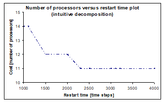Figure 7. Number of processors versus restart time by intuitive decomposition (sound source localisation)

The cost could be attempted to be reduced both by increasing the latency and by applying suitable decompositions. Some characteristic cases will be shown later.

The runtime of the HLS tool was extremely long in this mode (requiring about 18 hours on a contemporary PC), mostly because of the high number of elementary operations. The longest time has been taken by the force directed scheduling algorithm.

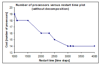Figure 8. Number of processors versus restart time without decomposition (sound source localisation)

4.2.  Results provided by DECHLS with preliminary decomposition for the sound source localization

In this experiment, DECHLS is applied using both task decompositions [21] based on the multilevel Kerrigan-Lin (KL) [23] algorithm and the spectral clustering (SC) [24]. The results are nearly the same. In both calculations, the desired number of segments has been prescribed as 5 and 7 respectively. Both results are illustrated in Fig. 9 and Fig. 10. In these figures and in the following ones, the relative segment execution times are also shown in small circle diagrams.

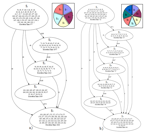Figure 9. Segment graphs resulted from KL decomposition (5 segments left, 7 segments right)

It is notable, that the results of different decomposition methods are almost the same. There are only minor differences in the segment contents and the execution times.

The third experiment on this benchmark is the application of DECHLS using the SC decomposition [24] algorithm without prescribing the number of segments. The SC algorithm is based on the lowest nonzero eigenvalues of the Laplacian matrix constructed from the graph [22], [30]. The lower eigenvalues we choose for the clustering, the smaller weight-sum will be caused by cut edges. Our applied version [22] does not make accessible

neither the Laplacian matrix, nor its eigenvalues. Therfore, we had to calculate them by applying a separate Matlab program. Since the Laplacian matrix is a square matrix with as many rows and columns as the number of nodes in the graph, the number of eigenvalues is also the same. Depending on the complexity of the graph to be decomposed, the larger eigenvalues may be extra large. Therefore, only the smallest 25 eigenvalues of the graph representing this example are shown in Fig. 11. Since the smallest 4 nonzero eigenvalues are identical, the most beneficial decomposition could result 4 segments.

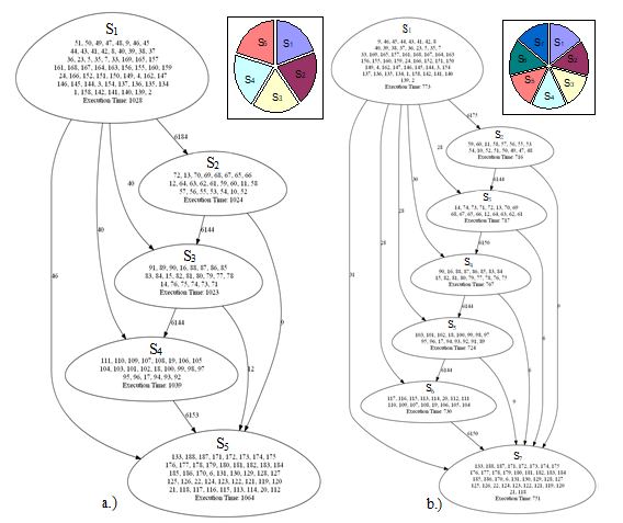Figure 10. Segment graphs resulted from spectral clustering decomposition (SC) (5 segments left, 7 segments right)

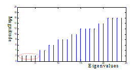Figure 11. Illustrating the smallest 25 eigenvalues of the Laplacian matrix used for decomposition

The result of this decomposition is shown in Fig. 12. It can be observed, that the sizes of the segments are not as uniform as in the previous cases. The reason of this is that the spectral clustering without local refinement cannot guarantee the approximately uniform segment sizes [21]. However, it is also notable, that the communication costs between the segments are now significantly lower.

Each of the resulting SGs (Figure 9, 10, 12) has been fed to our modified HLS tool in order to compute the cost versus restart time plots. Since the chosen decomposition method has a very small effect on the results, Fig. 9. a. is almost the same as Fig. 10. a. and Fig. 9. b. is almost the same as Fig. 10. b. Therefore, only three different diagrams are shown in Fig. 13.

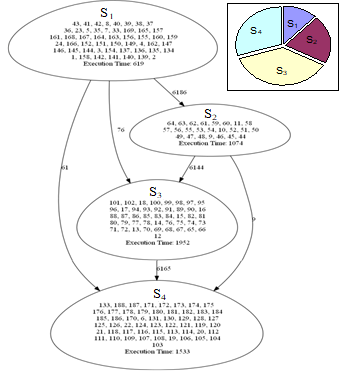Figure 12. Segment graph resulting from a spectral decomposition to 4 segments

4.3.  The effect of increasing the latency by DECHLS for the sound source localization

Figures 8 and 13 illustrate that DECHLS yields significantly less processors if preliminary decomposition is included. However it can be observed on this example (Fig. 9, 10, 12) that the latency became much longer (5178) by executing DECHLS with preliminary decomposition. The latency-increasing effect of the decomposition can be observed also even in the intuitively decomposed case (Fig. 4). Usually, the decomposition may have a latency- increasing effect. One of the reasons of this could be that operations assigned to the same segment can be executed only serially. If however, the modified HLS part is executed without preliminary decomposition, then much less serial constraints arise.

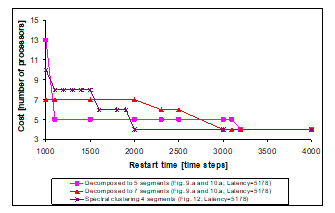Figure 13. Number of processors versus restart time plot after decomposition (sound source localisation)

On the other hand, a longer latency may influence advantageously the allocation and the restart time [18]. To illustrate this effect, the result of DECHLS without preliminary decomposition (Fig. 8) is recalculated (Fig. 14) at the increased latency value resulted with decomposition (Figures 9, 10, 12). In this example, further latency increasing would not have any remarkable effect, if the DECHLS is executed with preliminary decomposition as shown in Fig. 9, 10 and 12. Therefore such results are not shown in Fig. 14.

It can be observed in Fig. 14, that increasing the latency alone can provide acceptable costs, even assuming only identical processors, especially at restart time values greater than ca. 2000. The evaluation of the results in Fig. 14 would provide the most favourable solution achieved by the decomposition into 5 segments with the restart time 1100 (and the same number of processors as the number of segments in this case). However, if the restart time is less important than the cost, then the solution with 4 processors (decomposition into 4 segments by spectral clustering in this case) would be more beneficial.

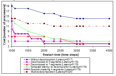Figure 14. Number of processors vs. restart time for comparison (sound source localisation)

4.4.  A high speed industrial data logger

The second benchmark for illustration is the redesign and evaluation of a high speed data logger [31] system (Fig. 15) that performs the measurement, pre-processing and storing of several different types of input data (i.e. temperature, pressure, humidity, and some other data measured by analogue sensors). The data are to be compressed before storing them in a serial memory. The frequency of sampling and storing is the same and constant for all kinds of data. In the existing system, this task is solved by low power 8 bit microcontrollers of the PIC18FxxKxx series. The data is stored in a relatively slow, but power efficient serial storage device accessible via the I2C bus. In each input, 4 channels for pressure, temperature and humidity sensing, and 8 channels for sensing other analogue signals are assumed. A possible dataflow graph of the system is shown in Fig. 15. The required sampling data rate is at least 10 samples per second that equals to 100ms pipeline restart time (initialization interval). The design goal is to find a cost-effective solution that complies with the data rate constraint. It will be assumed that the redesigned system also applies the same types of processors and storage device.

The pre-processing subtasks of the analogue input channels are supposed to be simple moving average filters. The pressure sensing and humidity sensing subtasks are more complex. Therefore their execution times are supposed to be much longer (Table 1). The reason of this is that these values need to be temperature compensated as a part of their pre-processing.

The existing solution applies three microcontrollers as component processors. The properties of the dataflow graph allow assigning identical subtasks per microcontrollers. The main advantage of this solution is to reuse the subroutines multiple times. However, it may make the system somewhat less efficient in speed and cost. The tasks of the processors are the following. P1 performs the measurement and pre-processing the data from 3 pressure sensors and from 2 humidity sensors. P2 measures and filters the data from 8 analogue sensors and from 4 temperature sensors, because both require the same filtering. P2 also measures the data from the remaining 2 humidity sensors and from one pressure sensor. A third microcontroller (P3) is used for temperature compensation of the pressure and humidity data and also for data compression and storing tasks. The whole system is pipelined so that P1 and P2 operate in parallel forming the first pipeline stage, while P3 works on the previous set of data as the next pipeline stage. The runtimes of subtasks assigned to P1 and P2 are critical; therefore a careful adjustment should be made in order to make these runtimes as close as possible to each other. This is shown in Table 1. The microcontrollers are supposed to communicate via their SPI serial interface at the maximal available speed (4MHz). So, the data communication time-step is 0.1 ms. In order to maximize the power efficiency, the clock speed of the microcontrollers is supposed to be fixed at 4MHz, i.e. 1 ms is 10 scheduling time steps. The above assumptions (summarized in Table 1.) may yield an intuitively designable pipeline system with a restart time (initialization interval) 69 ms (690 time steps), which meets the design criteria with about 14 samples per second. The latency is 108 ms (1080 time steps) in this case.

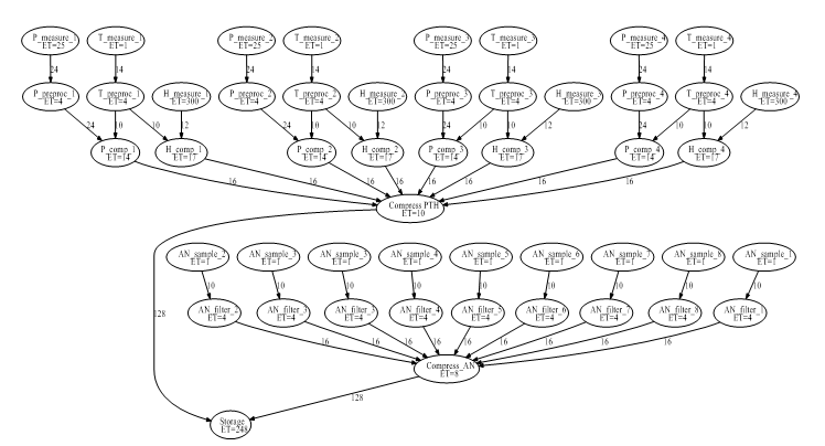Figure 15. Dataflow graph with execution times (time step is 0.1 ms) (high speed data logger)

Table 1. Runtime calculation for an intuitive design

Name of task	Execution time steps	Total number	Allocated to P1	Allocated to P2	Allocated to P3
AN_sample	1	8	0	8	0
AN_filter	4	8	0	8	0
P_measurement	25	4	3	1	0
H_measurement	300	4	2	2	0
T_measurement	1	4	0	4	0
P_comp	14	4	0	0	4
H_comp	17	4	0	0	4
P_preproc	4	4	3	1	0
T_preproc	4	4	0	4	0
Compress_PTH	10	1	0	0	1
Storage	248	1	0	0	1
Compress_AN	8	1	0	0	1
Total execution time (in time steps)		1766	687	689	390

4.5.  Evaluation of the existing decomposition for the high speed data logger

A carefully designed intuitive solution that complies with all the constraints was presented in Subsection 4.6. The intuitive decomposition is done firstly based on the parameter values in Table 1. The resulting segment graph is shown in Fig. 16.

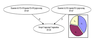Figure 16. Segment graph of the existing solution (high speed data logger)

In this implementation, the required number of processors is 3, the restart time is 690 time steps, and the latency is 1080 time steps. This intuitively designed system will be the basis for comparison.

4.6.  Results provided by DECHLS without decomposition for the high-speed data logger

Fig. 15 shows that the dataflow graph has such a special structure in this case, which causes less than 4 processors, only if the latency is increased from 570 to above 1400 time steps. This was calculated by the modified HLS tool. If the latency is increased to 1400 time steps (140 ms), then the solution is possible by applying 3 processors. However, this case requires a longer restart time, 1050 time steps (105 ms) than the prescribed value of 1000 (100 ms) given in Subsection 4.6.

4.7.  Results provided by DECHLS with preliminary decomposition for the high-speed data logger

Without prescribing the number of segments, the DECHLS yields 4 segments (Fig. 17 a). For comparison, 3, 4, 5 and 6 segments were prescribed by applying both KL and spectral clustering (SC) methods. For the sake of simplicity, only the following three cases from these are illustrated:

• 3 segments, KL method (Fig. 17. b)
• 3 segments, spectral clustering method, shortest restart time with 3 processors (Fig. 17. c)
• 5 segments, KL method, longest restart time with 3 processors (Fig. 17. d)

In this example, the number of segments and the selected decomposition method had greater influence on the results than in the sound source localisation example.

It is also notable, that the solution with 4 segments has the shortest latency, but not the longest restart time. However, the solution yielding the shortest restart time does not result in the longest latency. All of the above-mentioned cases are illustrated in Fig. 18.

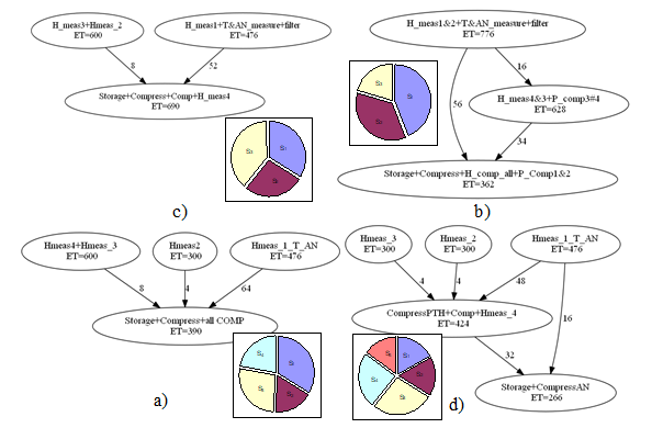Figure 17. Segment graphs and relative execution times obtained by some different decompositions (high speed data logger)

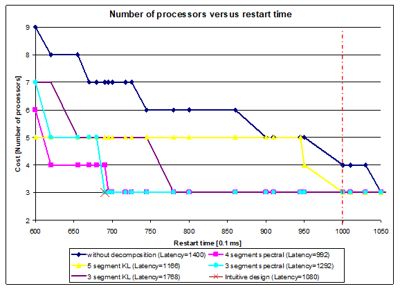Figure 18. Number of processors vs. restart time for comparison(high speed data logger)

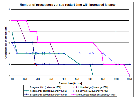Figure 19. Number of processors versus restart time with increased latency (high speed data logger)

4.8.  The effect of increasing the latency by DECHLS for the high speed data logger

In this example, the segment graphs yield significantly different latency values. Since increasing the latency may cause a not neglectable decrease in cost, it is worthy to analyze this effect. In the above presented cases, the longest latency time obtained is L=1768. For illustration, all other cases have been recalculated after increasing the latency to this value. The results are shown in Fig. 19.

It can be observed that the increased latency provides a more cost-efficient solution by applying the spectral clustering method producing 4 segments. This result can be considered the best one with only 2 processors with pipeline restart time 920, and with the latency value 1768. Note, that the cost became lower, but the restart time and the latency time values are worse than in the intuitive implementation. However, the design constraints set in Subsection 4.6 remained still fulfilled.

5. Conclusion

The system-level synthesis phase in designing multiprocessing systems can be supported by evaluating and comparing the solutions based on various numbers of processors in respect to desired properties of the system. In this paper, a method and an experimental tool (DECHLS) have been presented for generating various system-level structures. The method and the tool DECHLS are based on the combination of preliminary task decomposition and a modified high-level synthesis tool. In its present form, this combined method applies specific decomposition algorithms and a suitably modified high-level synthesis tool as components. These components can be modified or substituted by other ones according to the purpose of the designer or to the specific properties of the target system. The application of the tool DECHLS is illustrated on redesigning two existing multiprocessing systems by analyzing and evaluating the effects on various special requirements. For both examples, several alternative solutions were obtained by DECHLS, and the most characteristic results have been plotted as the cost (number of processors) against the pipeline throughput (as restarting period or initialization interval). Based on such considerations, the designer can select the most advantageous solutions regarding the priority order of cost, pipeline throughput and latency. For the presented specific constraints, some of the obtained solutions can be considered better than the existing system. The definition and calculation of the considered parameters can be modified by the user in DECHLS.

Acknowledgment

The research work presented in this paper has been supported by the Hungarian Scientific Research Fund OTKA 72611, by the “Research University Project” TAMOP IKT T5 P3 and the research project TAMOP-4.2.2.C-11/1/KONV-2012-0004.

1.  Gy. Racz, P. Arato, “A Decomposition-Based System Level Synthesis Method for Heterogeneous Multiprocessor Architectures“ IEEE System On Chip Conference, IEEE 2017, Munich, Germany https://doi.org/10.1109/SOCC.2017.8226082
2.  A. Gerstlauer, C. Haubelt, A. D. Pimentel, T. P. Stefanov, D. D. Gajski, J. Teich, “Electronic System-Level Synthesis Methodologies“, IEEE T COMPUT AID D., 28(10), 1517-1530, 2009
3.  R. Corvino, A. Gamatié, M. Geilen, L. Józwiak, “Design space exploration in application-specific hardware synthesis for multiple communicating nested loops“, in IEEE ICSAMOS, 128-135, 2012
4.  A. Carminati, R. S. de Oliveira, L. F. Friedrich, “Exploring the design space of multiprocessor synchronization protocols for real-time systems“, Journal of Systems Architecture (JSA), 60(3), 258-270, 2014. ISSN 1383-7621
5.  A. Cilardo, L. Gallo, N. Mazzocca, “Design space exploration for high-level synthesis of multi-threaded applications”, Journal of Systems Architecture (JSA), 59(10D), 1171-1183, 2013., ISSN 1383-7621
6.  P. Arató, Z. A. Mann, A. Orbán, “Finding optimal hardware/software partitions”, Formal Methods in System Design, 31(3), 241-263. 2007
7.  J. Wu, T. Srikanthan, G. Chen, “Algorithmic Aspects of Hardware/Software Partitioning: 1D Search Algorithms,” IEEE T. COMPUT., 59(4), 532-544, 2010. doi: 10.1109/TC.2009.173
8.  R. Ernst, J. Henkel, T. Benner, “Hardware-software cosynthesis for microcontrollers”, IEEE Design & Test of Computers, 10(4), 64-75, 1993.
9.  N. Govil, S. R. Chowdhury, “GMA: a high speed metaheuristic algorithmic approach to hardware software partitioning for Low-cost SoCs”, 2015 International Symposium on Rapid System Prototyping (RSP), Amsterdam, 2015.
10.  P. Arató, T. Visegrády, I. Jankovits, High Level Synthesis of Pipelined Datapaths, John Wiley & Sons, New York, ISBN: 0 471495582 4, 2001.
11.  W. Meeus, K. Van Beeck, T. Goedemé, J. Meel, D. Stroobandt, “An overview of today’s high-level synthesis tools”, Design Automation for Embedded Systems, 16(4), 31-51, 2012.
12.  T. Mukk, A. M. Rahmani, N. Dutt, “Adaptive-Reflective Middleware for Power and Energy Management in Many-Core Heterogeneous Systems”, International Symposium & Workshop on Many-Core Computing: Hardware and Software, Southampton, UK, 2018.
13.  P. Arató, Z. A. Mann, A. Orbán, “Time-constrained scheduling of large pipelined datapaths”, Journal of Systems Architecture (JSA), 51(12), 665-687, 2005.
14.  P. G. Paulin, J. P. Knight, “Force-directed scheduling for the behavioral synthesis of ASICs” IEEE T COMPUT AID D., 8(6), 661-679, 1989.
15.  M. Grajcar, “Genetic List Scheduling Algorithm for Scheduling and Allocation on a Loosely Coupled Heterogeneous Multiprocessor System”, 36th ACM/IEEE Conference on Design Automation, New Orleans, LA, USA, 1999.
16.  J-H. Ding, Y-T. Chang, Z-D. Guo, K-C. Li, Y-C. Chung, “An efficient and comprehensive scheduler on Asymmetric Multicore Architecture systems”, Journal of Systems Architecture, 60(3), 305-314, 2014, ISSN 1383-7621
17.  C-S. Lin, C-S. Lin, Y-S. Lin; P-A. Hsiung, C. Shih, “Multi-objective exploitation of pipeline parallelism using clustering, replication and duplication in embedded multi-core systems”, Journal of Systems Architecture (JSA), 59(10C), 1083-1094, 2013, ISSN 1383-7621
18.  Gy. Pilászy, Gy. Rácz, P. Arató, “The effect of increasing the latency time in High Level Synthesis”, Periodica Polytechnica Electrical Engineering, 58(2), 37-42, 2014. https://doi.org/10.3311/PPee.7024
19.  K. O’Neal, D. Grissom, P. Brisk, “Force-Directed List Scheduling for Digital Microfluidic Biochips”, IEEE/IFIP 20th International Conference on VLSI and System-on-Chip (VLSI-SoC), Santa Cruz, USA, 2012.
20.  P. G. Paulin, J. P. Knight, “Force-Directed Scheduling in Automatic Data Path Synthesis”, 24th Conference on Design Automation, New York, USA, 1987.
21.  P. Arató, D. Drexler, Gy. Rácz, “Analyzing the Effect of Decomposition Algorithms on the Heterogeneous Multiprocessing Architectures in System Level Synthesis” Buletinul Stiintific al Universitatii Politehnica din Timisoara Romania Seria Automatica si Calculatore / Scientific Buletin of Politechnica University of Timisoara Transactions on Automatic Control and Computer Science, 60(74) 39-46. 2015.
22.  B. Hendrickson, R. Leland, “The Chaco User’s Guide Version 2.0”, Technical Report SAND94-2692, 1994.
23.  B. Hendrickson, R. Leland, “A Multilevel Algorithm for Partitioning Graphs”, In Proc. Supercomputing ’95. (Formerly, Technical Report SAND93-1301), 1993.
24.  B. Hendrickson, R. Leland, “An Improved Spectral Graph Partitioning Algorithm for Mapping Parallel Computations”, SIAM J. Sci. Stat. Comput., 16(2), 452-469, 1995.
25.  G. Karypis, V. Kumar, “Metis-unstructured graph partitioning and sparse matrix ordering system version 2.0”, 1995.
26.  A. Trifunovic, W. J. Knottenbelt, “Parkway 2.0: a parallel multilevel hypergraph partitioning tool”, Computer and Information Sciences-ISCIS 2004, Springer, 789-800. 2004.
27.  M. Goraczko, J. Liu, D. Lymberopoulos, “Energy-Optimal Software Partitioning in Heterogeneous Multiprocessor Embedded Systems”, DAC 2008., Anaheim, California, USA, 2008.
28. G. Suba, “Hierarchical pipelining of nested loops in high-level synthesis”, Periodica Polytechnica Electrical Engineering, 58(3) 81-90, 2014. https://doi.org/10.3311/PPee.7610
29.  J. Subhlok, G. Vondran, “Optimal latency – throughput tradeoffs for data parallel pipelines”, 8th Annual ACM Symposium on Parallel Algorithms and Architectures, Padua, Italy, 1996.
30.  C. J. Alpert, A. B. Kahng, S.-Z. Yao, “Spectral partitioning with multiple eigenvectors”, Discrete Applied Mathematics, 90(1), 3-26, 1999.
31.  Project documentation of KMR_12-1-2012-0222 titled “The development of a complex monitoring system for fishing waters”

(Click Here)

(Click Here)