1. Introduction

Our research is an extension of work originally presented in the 2018 IEEE ICCAR Conference [1]. Many complex systems, such as energy consumption systems and transportation systems, involve both engineered and non-engineered system factors. For example, the energy consumption system of a building involves both engineered system factors, (e.g., AC equipment, pump for water use, lighting system, computers, and network equipment) and non-engineered system factors, (e.g., social/behavioral factors, such as occupants’ activities, and environmental/natural factors such as outside climate), which are intertwined to drive the energy consumption and demand of the building [2-4]. For another example, the transportation system involves both engineered system factors, (e.g., the transportation infrastructure including highways, streets and roads, and traffic control mechanisms, such as traffic lights) and non-engineered system factors, (e.g., social/behavioral factors such as traffic flows, drivers, pedestrians, and car accidents, as well as natural/environmental factors, such as weather conditions).

Although models of engineered systems may be available, models of mixed-factor systems are usually not available due to unknown interconnectivities and interdependencies of many engineered and non-engineered system factors. A complete, accurate system model, which clearly defines relations of system variables including interconnectivities and interdependencies of engineering and non-engineered system factors, is highly desirable for many applications. For example, variable relations of energy consumption are required to enable the accurate estimation of energy consumption/demand and the close alignment of energy production with energy demand to achieve energy production and use .

Utility/energy companies currently rely heavily on the past data of electricity loads in base, average and peak to project energy production/supply. This statistical investigative activity is done without adequate and accurate models of energy consumption systems [3]. Power plants often generate enough power to satisfy base loads and meet the difference between peak and base loads, sudden demand surge or any gap of energy supply and demand through their excess production capacities or by procuring from other energy sources [5, 6]. Historical data lack critical real-time features (e.g., the lag effect of historical data, and lack of finer levels and finer divisions in time and space) for the accurate projection and estimation of energy demand and consumption. Without adequate and accurate models of energy consumption systems, it is extremely difficult to obtain an accurate projection and estimation of energy demand and consumption. As a result, energy has to be produced in excess in order to meet potential rise in demand. Energy production in excess is a significant cause of waste and inefficiency. Even with current technologies to obtain dynamic data of energy consumption systems in real time, the lack of adequate and accurate energy system models renders real-time dynamic system data useless for closely aligning energy production with energy demand to achieve energy production efficiency and energy use reduction. The ultimate energy efficiency through smart energy production and use will enable a shift from the existing code-, standard- and experience-based forecasting approach to a more dynamic, real-time and smart technology environment based on real-time data, models and analytics for the real-time, accurate estimation of energy consumption and smart technologies to align energy production with energy demand closely for energy use reduction and energy production efficiency.

Many statistical modeling, data mining and machine learning techniques for system modeling, including decision trees, regression analysis, artificial neural network, and Bayesian networks, have been used to analyze and model energy consumption and efficiency of equipment, homes and buildings [7-16]. System modeling techniques based on many existing statistical analysis, machine learning and data mining have a shortcoming of building variable relations for the full ranges of variable values using one model, although certain variable relations may hold for only some but not all variable values. This shortcoming is overcome by the PVAD algorithm that is a new multivariate analysis algorithm to learn both full-value and partial-value relations of system variables from system data. Our research used the PVAD algorithm to model variable relations of energy consumption from data by learning full-and partial-value variable relations of energy consumption. The PVAD algorithm was applied to building energy consumption data at ASU.

2. Shortcomings of existing techniques of system modeling from data

Existing methods of learning system models from data include statistical analysis [17-24] and data mining techniques [23-32]. With system modeling from data, classification and prediction can be performed to explain or find relations among system variables. Depending on the nature of data, there are several methods to analyze data using statistical techniques such as parametric, non-parametric and logistic regression. For example, when modeling categorical dependent variables, logistic regression can be applied [17, 21, 22]. In addition to decision and regression trees [23, 24], random forest and support vector machine are also considered [25-28, 29, 31]. However, the above methods assume that the role of a variable in a variable relation is known (i.e., which variable is an independent or dependent variable) and a variable plays only one role of being either an independent variable or a dependent variable in one layer of variable relations. Once a variable is considered as an independent variable, it can no longer be utilized as a dependent variable which is a main disadvantage especially when the role of a variable is not known or when multiple layers of variable relations are required where a variable can play different roles of being an independent or dependent variable in different variable relations at different layers.

Bayesian networks [23, 24, 35-37], structural equation models [33, 34] and reverse engineering methods [38-47] are examples of a few options left that can provide system modeling without prior knowledge of variables. However, those techniques discover only variable relations for full ranges of all  variable values instead of relations for specific values only. This can be seen from the Fisher’s Iris data set [48] in which the classification of the target variable (Plant Type) using independent variables works for only the values of Iris Versicolor and Iris Virginica) for the target variable but not for another target value of Iris Sentosa. For such data where variable relations hold for partial ranges of variable values only or different variable relations hold for different ranges of variable values, the model of the same variable relations for all variable values do not fit all data values well, that is, the model explains or represents the whole data set poorly.

The PVAD algorithm was developed as a new system modeling technique [49-51] to overcome the above shortcomings. Variable value associations can be used to construct associative networks as multi-layer structural system models. The application of the PVAD based system modeling technique is part and parcel of our research of energy consumption in systems.

3. The energy consumption data and the PVAD application

      The PVAD algorithm is presented in detail in [49-51]. This section shows the PVAD application to data of energy consumption collected from an ASU building in January 2013 for modeling energy consumption. There was a data sample every 15 minutes. The data set has 2976 data records or instances. Each data record contains four numeric values for the consumption of electricity (E), cooling (C), heating (H), and air temperature (A), respectively, as well as TimeStamp (T). T is important because changes of T are associated with changes in presence and activities of occupants and changes of E, C and H.

To apply the PVAD algorithm, in Step 1 the numeric variables of A, H, C, and E, were transformed into categorical variables as shown in Fi To apply the PVAD algorithm, in Step 1 the numeric variables of A, H, C, and E, were transformed into categorical variables as shown in Figures (1)-(4). More details of Step 1 are in [1].

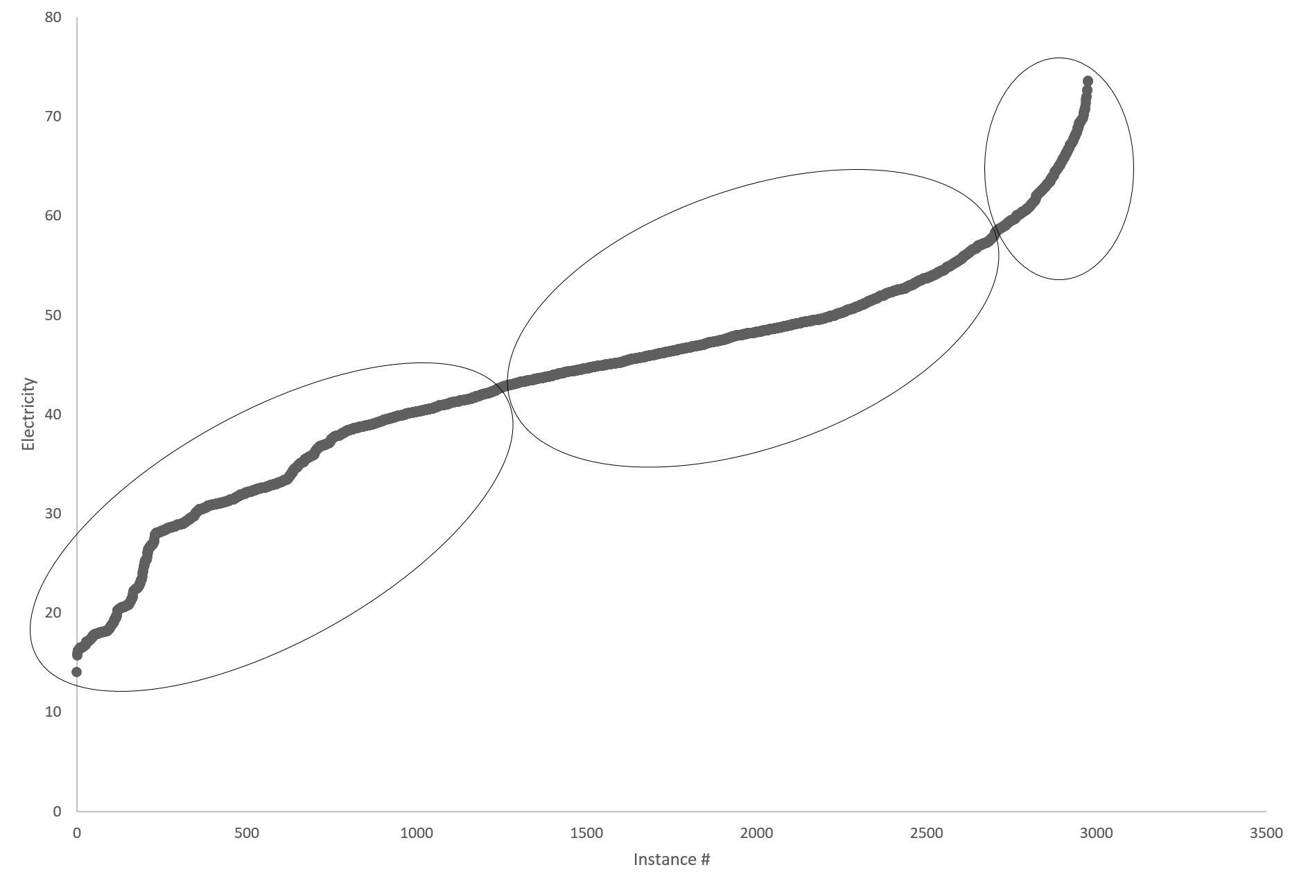Figure 1. An example of plotting E values to determine data clusters and categorical values.

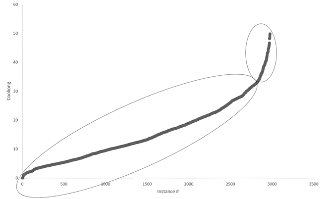Figure 2. An example of plotting C values to determine data clusters and categorical values.

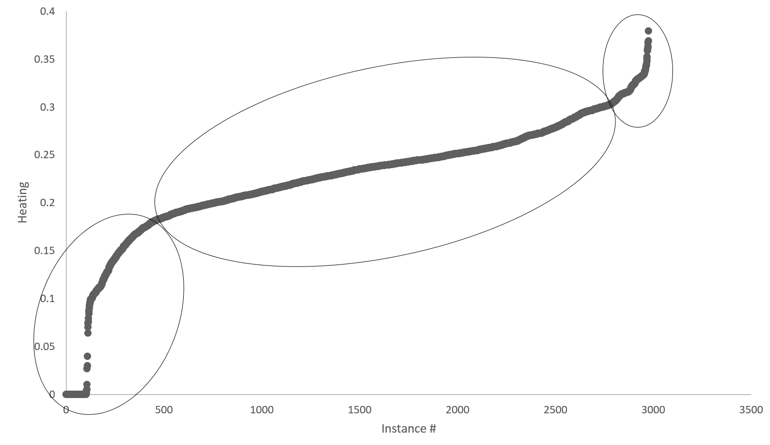Figure 3. An example of plotting H values to determine data clusters and categorical values.

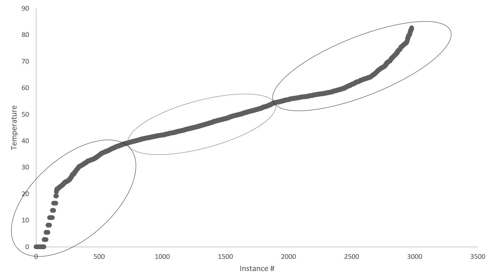Figure 4. An example of plotting A values to determine data clusters and categorical values.

Step 2.1 generated candidate 1-to-1 associations of partial variable values, x = a à y = b, where x = a is the conditional variable value (CV) and y = b is the associative variable value (AV), and computed the co-occurrence ratio (cr) of each candidate association as follows:

If cr is greater than or equal to the parameter α, we had an established association. For example, Table (1) shows 1-to-1 associations having  CV: C = High together with their respective cr values and α = 0.8.

Table 1: 1-to1 associations of ASU energy consumption data with CV: C=High

#	Association	cr	Co-Occurrence Frequency ( )	Type of Association
1	C=High à T=12:15 PM to 5:30 PM	0.48	62	Candidate
2	C=High à T=5:45 PM to 11 PM	0.43	55	Candidate
3	C=High à T=8:15 AM to 12 PM	0.09	11	Candidate
4	C=High à E=High	0.20	25	Candidate
5	C=High à E=Medium	0.80	103	Established
6	C=High à H=Low	0.73	94	Established
7	C=High à H=Medium	0.27	34	Candidate
8	C=High à A=High	0.96	123	Established
9	C=High à A=Medium	0.04	5	Candidate

In addition to parameter α, two other parameters, β and γ, are also needed. β is used to remove associations whose number of supporting instances (the instances containing variable values in the numerator of equation 1) is smaller than β. γ is used to remove an association with a common CV or AV that appears in more than γ of the data set. In this example, β is set to be 50 while α and γ are set to 0.8 and 0.95, respectively.

Step 2.2 uses two methods, YFM1 and YFM2, to examine and esyablish p-to-q associations, X = A à Y = B, where X and Y represent multiple variables. For example, using #5, 6 and 8 in Table (1), we applied YFM1 which considers all combinations of AVs covered in those associations so as to find 1-to-q associations, where q >1. To find 1-to-2 established associations, we first computed  Then we considered all possible combinations of two-variable AVs from the established 1-to-1 associations:

1. C=High->E=Medium, H=Low (from #5 and #6)
2. C=High->E=Medium, A=High (from #5 and #8)
3. C=High->H=Low, A=High (from #6 and #8).

For each 1-to-2 candidate associations above, , the number of instances in the common subset of supporting instance, was computed to calculate cr for the 1-to-2 association. The results are given in Table (2). In this case, C=High->H=Low, A=High is the only established association.

Table 2: Calculation for 1-to-2 associations with CV: C=High

#	Association		cr  / 128)
1	C=High à E=Medium, H=Low	87	0.6796875
2	C=High à E=Medium, A=High	103	0.125
3	C=High à H=Low, A=High	94	0.8046875

YFM2 is used to find 2-to-1 associations. YFM2 considers all candidate associations (cr value in (0, 1]) not just established associations (cr . Table (3) is used to illustrate YFM2 in the following.

• Determine . If we pick C=High->T=12:15 PM to 5:30 PM to start with, Then 50 and the 2-to-1 association that we would like to generate will have C=High, T=12:15 PM to 5:30 PM as CV. Note that if , the whole group is dropped as the number of instances covered by the new CV is just the occurrence frequency which should be .

2i)   Iterate through all other associations from Table (2). Skip immediately to the next line if the AV of that association is the same as one picked in the previous step. For example, #2 has AV: T=5:45 PM to 11 PM that represents Timestamp. While the AV of the association also represents timestamp (T=12:15 PM to 5:30 PM), we skip to #3 without looking at the intersection of the instances.

2ii)  Generate 2-to-1 association if n_intersection ≥ 50. Table (3) lists the n_intersection and the corresponding cr value.

Table 3: Calculation for 2-to1 associations of ASU energy consumption data with CV “C=High, T=12:15 PM to 5:30 PM”

Combination (Type of Association)	Association		cr  )
1 & 4 (Candidate)	C=High, T=12:15 PM to 5:30 PM à E=High	3	0.04
1 & 5 (Established)	C=High, T=12:15 PM to 5:30 PM  à E=Medium	59	0.9516
1 & 6 (Candidate)	C=High, T=12:15 PM to 5:30 PM  à H=Low	59	0.9516
1 & 7 (Candidate)	C=High, T=12:15 PM to 5:30 PM à H=Medium	3	0.04
1 & 8 (Established)	C=High, T=12:15 PM to 5:30 PM à A=High	62	1
1 & 9 (Candidate)	C=High, T=12:15 PM to 5:30 PM à A=Medium	0	0

Following the same procedure, other p-to-q associations were generated by YFM1 and YFM2. Step 3 generalized and consolidated variable associations of partial values into associations of full value ranges if there are partial-value associations covering the full value range of the same variable.

The PVAD algorithm was used to analyze the energy consumption data using various values of α = 1, 0.9, and 0.8, β = 50, 30, and 10, and γ = 95%. The results for γ = 95%, β = 50, and α = 0.8 are most meaningful and presented in the next section.

4. Results of the PVAD Algorithm

Tables (4)-(5) list the most specific association(s) in each group of the associations with the same AV. Table (6) lists the most generic association(s) in each group of the associations with the same AV. Variable relations for energy consumption revealed by each association in Tables (4)-(6). In Tables (4)-(6), there are groups that give similar associations. For example, the associations in Group 1 and Group 2 in Table (6) are similar. For the groups with similar associations, we marked only one group using the symbol ^ in the column of group #. Most of the associations in Tables (4)-(6) involve C=Low for cooling being low in CV or AV, because most of instances in the data set (2848 out of totally 2976 instances) contain C=Low due to the month of January when the data was collected. Since C=Low is so common in the data set, C=Low can be dropped from the associations when interpreting associations.

Table 4: Specific associations in each group of associations with the same AV: Set 1

Group #	The most specific association(s) in group
1	A=Medium, [ T=12:15 PM to 11 PM, E=High]/ [ T=6:15 AM to 11 PM, E=Medium]/[T=11:15 PM to 6 AM, E=Low] à H=Medium, C=Low
2^	A=Medium, C=Low, [T=11:15 PM to 6 AM, E=Low]/[T=6:15 AM to 12 PM, E=Medium]/[T=12:15 PM to 11 PM, E=High/Medium] à H=Medium A=High, C=Low, E=Medium, T=8:15 AM to 12 PM à H=Medium
3^	A=High, E=Medium, C=High, T=12:15 PM to 5:30 PM à H=Low
4	C=High, E=Medium, T=12:15 PM to 5:30 PM à A=High | H=Low
5^	H=High, E=Medium, T=6:15 AM to 8 AM à A=Low, C=Low
6	H=Medium, E=Low, T=12:15 PM to 5:30 PM à A=High, C=Low
7^	[E=Medium, C=*, H=Low]/[E=Low, C=Low, H=Medium], T=12:15 PM to 5:30 PM à A=High C=High, T=5:45 PM – 11 PM à A=High
8	H=Medium, E=High, T=12:15 PM to 5:30 PM à A=Medium, C=Low
9^	H=Medium, C=Low, E=High, T=12:15 PM to 5:30 PM, à A=Medium
10	H=High, C=Low, E=Medium, T=6:15 AM to 8 AM, à A=Low
11^	[A=Low, H=High]/[ A=High, H=Low]/[ A=Low/Medium, H=Medium], C=Low, T=11:15 PM to 6 AM à E=Low
12	[A=Low, H=High]/[A=High, H=Low]/[A=Medium/Low, H=Medium], T=11:15 PM to 6 AM à C=Low, E=Low

Table 5: Specific associations in each group of associations with the same AV: Set 2

13	A=Medium, H=High, T=5:45 PM to 11 PM à C=Low, E=Medium T=8:15 AM to 12 PM, H=Medium, A=High/Medium à E=Medium, C=Low
14^	A=High, H=Low, C=High, T=12:15 PM to 5:30 PM à E=Medium A=Medium, H=High, C=Low, T=5:45 PM to 11 PM à E=Medium A=Medium/High, H=Medium, C=Low, T=8:15 AM to 12 PM à E=Medium
15	H=Low, C=High, T=12:15 PM to 5:30 PM à A=High | E=Medium
16^	A=High, C=High, T=12:15 PM to 5:30 PM, à H=Low | E=Medium A=Medium/High, C=Low, T=8:15 AM to 12 PM à H=Medium | E=Medium

The associative network of the energy consumption system model shown in Figure (5) was constructed using the associations in the groups marked with ^ in Table (6). Figure (5) shows the factors associated with the high, medium and low air temperatures (from the associations with A as the AV), the factors associated with the Medium and Low heating consumption (from the associations with H as the AV), and the factors associated with the medium and low electricity consumption (from the associations with E as the AV).

Figure (5) shows that E, C, H and A are related differently in different time periods. For example, in the afternoon, T = 12:15 PM to 5:30 PM, the medium heating consumption (H = Medium) along with the high electricity consumption (E = High) is associated with the medium air temperature (A = Medium), whereas in the early morning, T = 6:15 AM to 8 AM, the high heating consumption (H = High) is associated with the low air temperature (A = Low). Similarly, the most specific associations in Tables (4)-(5), even the most generic associations in Table (6) and in Figure (5) show that associations of T, E, C, H and A differ in different value ranges of these variables. This illustrates that the PVAD algorithm can discover full/partial-value variable relations that exist in many real-world systems.

Table 6: Generic associations in each group of associations with the same AV.

Group #	The most generic association(s) in each group
1^	A=Medium/E=High à H=Medium
2	E=High/A=Medium, C=Low à H=Medium
3	E=Medium, C=High, A=High à H=Low
4	E=Medium, C=High à H=Low | A=High
5^	H=High, T=6:15 AM to 8 AM à A=Low.
6^	E=Low, T=12:15 PM to 5:30 PM à A=High
7^	H=Low à A=High T=5:45 PM – 11 PM, C=High à A=High C=Low, E=Low, T=12:15 PM to 5:30 PM à A=High
8^	H=Medium, E=High, T=12:15 PM to 5:30 PM à A=Medium
9	H=Medium, C=Low, E=High, T=12:15 PM `to 5:30 PM à A=Medium
10	H=High, C=Low, T=6:15 AM to 8 AM à A=Low
11	C=Low, T=11:15 PM to 6 AM à E=Low
12^	T=11:15 PM to 6 AM à E=Low
13^	T=8:15 AM to 12 PM à E=Medium H=High, T=5:45 PM to 11 PM à E=Medium
14	H=High, C=Low, T=5:45 PM to 11 PM à E=Medium C=High à E=Medium
15	C=High à A=High | E=Medium
16^	A=High, C=High, T=12:15 PM to 5:30 PM à H=Low | E=Medium A=Medium/High, C=Low, T=8:15 AM to 12 PM à H=Medium | E=Medium

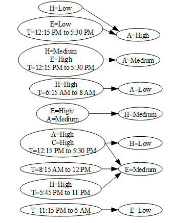Figure 5. The most generic associations in the groups marked by ^ in Table (6) represented in an associative network.

5. Comparison of the PVAD algorithm with some data mining techniques

We considered two of the existing data mining techniques to compare with the PVAD algorithm: association rule and decision tree.

5.1. Comparison with the association rule technique

The association rule technique first uses the Aprori algorithm to determine frequent item sets that satisfy the minimum support [23-24]. Then each frequent item set is broken up into all possible combinations of association rules which are evaluated to see if any of them satisfy the minimum support and confidence. For a large dataset, frequent item sets and candidate association rules from frequent item sets can be enormous, requiring huge amounts of computer memory space and computation time. When the association rule technique was applied to the energy consumption data, there were too many frequent item sets and consequently association rules to be listed in this paper. While the performance of the association rule technique was hindered by the data size, the search space of associations in the PVAD algorithm is narrowed down by YMF1 and YFM2, along with parameters α, β and γ.

5.2 Comparison with the decision tree technique

Decision tree is a data mining technique to learn decision rules that express relations of the dependent variable y with independent variables x in a directed and acyclic graph [23-24]. The software, Weka, was used to construct decision trees of the energy consumption system data, To construct a decision tree in Weka, there are different algorithms such as ID3 [52] and J48 [53]. The later one is an extended version of ID3 with additional features like dealing with missing values and continuous attribute value ranges. It also addresses the over-fitting problem that decision trees are prone to by pruning. The pruning process requires the computation of the expected error rate. If the error rate of a subtree is greater than that of a leaf node, a subtree is pruned and replaced by the leaf node.

In our research, ID3 was used for the comparison with the PVAD algorithm because ID3 produces comparable results with associations produced by the PVAD algorithm. Leaf nodes produced by ID3 are pure in that the class labels of instances are the same in each leaf node. The purity of leaf node corresponds to AV in associations from the PVAD algorithm having the same variable value. The PVAD algorithm produces all associations up to N-to-1 associations, where N+1 is the number of variables. In other words, the PVAD algorithm can generate the longest CVs and find the AV that they are associated with. The combination of CVs corresponds to the path from the root of a decision tree down to a leaf node.

Because the decision tree technique requires the identification of one dependent variable (the target variable) and independent variables (attribute variables) for each decision tree, five decision trees need to be constructed for each of the five variables as the dependent variable. Tables (7)-(10) list decision rules produced by one of the five ID3 trees.

Although the decision rules from the decision trees appear to have the same form as associations from the PVAD algorithm, a decision rule has a different meaning from an association from the PVAD algorithm. A decision rule derived from the root of a decision tree to a leaf node of the decision tree represents a frequent item set with instances in the leaf node having the values of the target variable and the attribute variables in the decision rule. This is why we see a path in a decision tree is also present in another tree even though different decision trees have different target variables. For example, the variable values in E=Medium, A=High, H=Medium, C=Low, T=12:15 PM to 5:30 PM, are found in all four decision trees. Note that the energy consumption data set has only five variables. Redundant paths of different decision trees can be found more often for larger data sets with more variables. This means the waste of computation time and space and the difficulty of sorting  out results from a  number  of

Table 7: Decision rules from the ID3 Tree with Air Temperature as the target variable same as PVAD association rules

#	Decision rules that appear same as PVAD association rules
1	H=Medium, E=High, T=12:15 PM to 5:30 PM à A=Medium
2	H=Medium, E=Low, T=12:15 PM to 5:30 PM à A=High
3	H=Low, T=12:15 PM to 5:30 PM à A=High
4	H=High, E=Medium, T=6:15 AM to 8 AM à A=Low

Table 8: Decision rules from the ID3 Tree with Air Temperature = Low as the target variable

5	H=Medium, E=High, T=11:15 PM to 6 AM à A=Low
6	H=High, E=Low, T=11:15 PM to 6 AM à A=Low
7	H=High, E=Medium, T=11:15 PM to 6 AM àA=Low
8	H=High, E=Medium, T=12:15 PM to 5:30 PM à A=Low
9	H=High, E=Low, T=6:15 AM to 8 AM à A=Low
10	H=Medium, E=Low, T=6:15 AM to 8 AM à A=Low
11	H=High, E=Low, T=8:15 AM to 12 PM à A=Low
12	H=High, E=Medium, T=8:15 AM to 12 PM à A=Low
13	H=Low, C=Low, E=Medium, T=5:45 PM to 11 PM à A=Low

Table 9: Decision rules from the ID3 Tree with Air Temperature = Medium as the target variable

14	H=Low, T=6:15 AM to 8 AM à A=Medium
15	H=Medium, E=Low, T=11:15 PM to 6 AM à A=Medium
16	H=Low, E=Medium, T=11:15 PM to 6 AM à A=Medium
17	H=Medium, E=Medium, T=11:15 PM to 6 AM à A=Medium
18	H=High, E=Low, T=12:15 PM to 5:30 PM à A=Medium
19	H=High, E=Low, T=5:45 PM to 11 PM à A=Medium
20	H=High, E=Medium, T=5:45 PM to 11 PM à A=Medium
21	H=Medium, E=Medium, T=6:15 AM to 8 AM à A=Medium
22	H=Medium, E=High, T=8:15 AM to 12 PM à =Medium
23	H=Medium, E=Low, T=8:15 AM to 12 PM à A=Medium
24	H=Medium, C=Low, E=High, T=5:45 PM to 11 PM à A=Medium
25	H=Medium, C=Low, E=Medium, T=5:45 PM to 11 PM à A=Medium
26	H=Medium, C=Low, E=Medium, T=8:15 AM to 12 PM à A=Medium

decision trees. Hence, a decision rule corresponds to a frequent item set in the association rule technique, whereas an association from the PVAD algorithm corresponds to an association rule in the association rule technique. This is why there are decision rules in Tables (7) – (10) that are not found in associations of the PVAD algorithm because frequent item sets for those decision rules were eliminated in the process of forming associations. Hence, the PVAD algorithm has the advantage to the decision tree technique because the PVAD algorithm discovers associations rather than frequent item sets.

Table 10: Decision rules from the ID3 Tree with Air Temperature = High as the target variable

27	H=Low, E=Low, T=11:15 PM to 6 AM à A=High
28	H=Low, E=High, T=5:45 PM to 11 PM à A=High
29	H=Low, E=Low, T=5:45 PM to 11 PM à A=High
30	H=Low, E=Low, T=8:15 AM to 12 PM à A=High
31	H=Medium, C=High, E=High, T=5:45 PM to 11 PM à A=High
32	H=Medium, C=Low, E=Low, T=5:45 PM to 11 PM à A=High
33	H=Low, C=High, E=Medium, T=5:45 PM to 11 PM à A=High
34	H=Medium, C=High, E=Medium, T=5:45 PM to 11 PM à A=High
35	C=High, H=Low, E=Medium, T=8:15 AM to 12 PM à A=High
36	H=Medium, C=High, E=Medium, T=8:15 AM to 12 PM à A=High
37	H=Low, C=Low, E=Medium, T=8:15 AM to 12 PM à A=High
38	H=Medium, C=High, E=Medium, T=12:15 PM to 5:30 PM à A=High
39	H=Medium, C=Low, E=Medium, T=12:15 PM to 5:30 PM à A=High

There is another difference between the decision tree technique and the PVAD algorithm. Each step of constructing a decision tree performs the splitting of a data subset for data homogeneity based on the comparison of splits using only one variable and its values rather than combinations of multiple variables due to the large number of combinations and the enormous computation costs. Hence, the resulting decision tree contains decision rules with the consideration of only one variable at a time and may miss decision rules that can be generated if multiple variables and their values are considered and compared at a time. However, the PVAD algorithm examines one to multiple variables at a time and does not miss any associations that exist. The PVAD algorithm thus has the advantage to the decision tree technique by not missing any established associations and using YFM1 and YFM2 to cut down the computation costs.

Moreover, the decision tree algorithm requires the identification of the dependent variable (the target variable) and the independent variables (the attribute variables) although there may no priori knowledge for the identification of which variable is a dependent or independent variable. This is why five decision trees, with one decision tree taking each of the five variables as the target variable, had to be constructed for the energy consumption data. The PVAD algorithm does not require the distinction of dependent and independent variables but discovers variable value relations and the role of each variable in each variable value relation.

Furthermore, the PVAD algorithm can generate p-to-q associations with q > 1 that the decision tree technique cannot generate because a decision tree is constructed for only one target variable and produces only p-to-1 decision rules. Given the differences of the PVAD algorithm and the decision tree technique, the results of the PVAD algorithm are not comparable to the results of the decision tree technique. As discussed in Section 2, the PVAD algorithm overcomes shortcomings of existing statistical analysis and data mining techniques and produce partial/full-value associations that cannot be produced from other existing techniques.

5. Conclusion

Our research used the PVAD algorithm to learn and build the system model of energy consumption from data, especially learn relations of variables for both full and partial value ranges. The resulting partial-value associations of variables in the energy consumption system model reveal variable relations for partial value ranges that require not one but different models of variable relations over full value ranges of the variables. This finding shows that the PVAD algorithm has the advantage and capability of discovering variable relations for building a multi-layer, structural system model. Hence, the PVAD based system modeling technique can be useful in many fields to learn system models from data. The advantages of the PVAD algorithm to existing data mining, machine learning and statistical analysis techniques were also demonstrated by comparing the PVAD algorithm and its results from the application to the energy consumption data with the association rule technique and the decision tree technique.

1. N. Ye, T. Y. Fok, X. Wang, J. Collofello, N. Dickson, “Learning partial-value variable relations for system modeling”, In Proceedings of the 2018 IEEE ICCAR Conference, Auckland, New Zealand, April 20-23,2018, https://ieeexplore.ieee.org/xpl/tocresult.jsp?isnumber=8384628.
2. Kwok, K green buildings: A comprehensive study of. Y. G., Statz, C., Wade, B., and Chong, W. K., “Carbon emissions modeling for calculation methods”, ASCE Proceeding of the ICSDEC (ICSDEC), 118-126, 2012, https://doi.org/10.1061/9780784412688.014.
3. Swan, L. G., V. I. Ugursal, “Modeling of end-use energy consumption in the residential sector: A review of modelling techniques” Renewable and Sustainable Energy Reviews (Sust. Energ. Rev), 13(8), 1819-1835, 2009.
4.  Zhao, H.-X., Magoulès, F., “A review on the prediction of building energy consumption” Renewable and Sustainable Energy Reviews (Renew. Sust. Energ. Rev.), 16(6), 3586-3592, 2012.
5. PSC Wisconsin, Electricity Use and Production Patterns. Public Service Commission of Wisconsin. Madison, WI: Public Service Commission of Wisconsin. Retrieved from https://psc.wi.gov/thelibrary/publications/electric/electric04.pdf., 2011.
6. Flex Alert., Peak Demand. Retrieved from Flex Alert Home: http://www.flexalert.org/energy-ca/peak., 2013.
7. Ahmed, A., et al. Ahmed, A., et al., “Mining building performance data for energy-efficient operation” Advanced Engineering Informatics (Adv. Eng. Inform)., 25(2), 341-354, 2011.
8. Berges, M. E., et al. “Enhancing Electricity Audits in Residential Buildings with Nonintrusive Load Monitoring”, Journal of Industrial Ecology (J. Ind. Ecol.), 14(5), 844-858, 2010.
9. Fan, C., et al., “Development of prediction models for next-day building energy consumption and peak power demand using data mining techniques” Applied Energy (Appl. Energ.), 127(0), 1-10, 2014.
10. Hawarah, L., et al., User Behavior Prediction in Energy Consumption in Housing Using Bayesian Networks, Artificial Intelligence and Soft Computing, Springer Berlin Heidelberg, 6113: 372-379, 2010.
11. Khan, I., et al., “Fault Detection Analysis of Building Energy Consumption Using Data Mining Techniques” Energy Procedia (Enrgy. Proced.), 42, 557-566, 2013.
12. Khansari, N., et al., “Conceptual Modeling of the Impact of Smart Cities on Household Energy Consumption” Procedia Computer Science (Procedia. Comput. Sci.), 28, 81-86, 2014.
13. Kim, H., et al., “Analysis of an energy efficient building design through data mining approach”, Automation in Construction (Automat. Constr.), 20(1), 37-43, 2011.
14. Palizban, O., et al., “Microgrids in active network management – part II: System operation, power quality and protection”, Renewable and Sustainable Energy Reviews (Renew. Sust. Energ. Rev.), 2014.
15. Tso, G. K. F. and K. K. W. Yau, “Predicting electricity energy consumption: A comparison of regression analysis, decision tree and neural networks”, Energy, 32(9), 1761-1768, 2007.
16. Vollaro, R. D. L., et al., “An Integrated Approach for a Historical Buildings Energy Analysis in a Smart Cities Perspective” Energy Procedia (Enrgy. Proced.), 45(0), 372-378, 2014.
17. Friedman, J. H., “Multivariate Adaptive Regression Splines”, The Annals of Statistics ( Stat.), 1-67, 1991.
18. Hastie, T., Tibshirani, R., and Friedman, J. H. The Elements of Statistical Learning, 2nd edition. New York, New York: Springer,
19. Zhang, H., and Singer, B. H., Recursive Partitioning and Applications, 2nd edition. New York, New York: Springer, 2010.
20. Freedman, D. A., Statistical Models: Theory and Practice. Cambridge University Press, 2009.
21. Bishop, C. M., Pattern Recognition and Machine Learning. Springer,
22. James, G., Witten, D., Hastie, T., and Tibshirani, R., An Introduction to Statistical Learning. Springer,
23. Ye, N., Data Mining: Theories, Algorithms, and Examples, Boca Raton, Florida: CRC Press,
24. Ye, N., The Handbook of Data Mining. Mahwah, New Jersey: Lawrence Erlbaum Associates,
25. Gasse, M., Aussem, A., and Elghazel, H., An experimental comparision of hybrid algorithms for Bayesian network structure learning. Lecture Notes in Computer Science: Machine Learning and Knowledge Discovery in Databases, 7523: 58-73.,
26. Breiman, L., “Random forests” Machine Learning (Mach. Learn.), 45(1), 5–32, 2001
27. Breiman, L., “Arcing classifier”, Statist (Ann. Stat.), 26(3), 801–849, 1998.
28. Breiman, L., “Bagging predictors”, Machine Learning (Mach. Learn.), 24(2), 123–140, 1996.
29. Freund, Y., and Schapire, R. E., “Decision-theoretic generalization of on-Line learning and an application to boosting”. Journal of Computer and System Sciences (J. Comput. Syst. Sci.), 55(1), 119-139, 1997.
30. Ho, T. K. “The random subspace method for constructing decision forests”, IEEE Transactions on Pattern Analysis and Machine Intelligence (IEEE T. Pattern. Anal.), 20(8), 832–844, 1998.
31. Kam, H. Tim., “Random decision forest.”, Proceedings of the 3rd International Conference on Document Analysis and Recognition, 1, 278-282, 1995.
32. Mason, L., Baxter, J., Bartlett, P. L., & Frean, M. R., “Boosting algorithms as gradient descent” Advances in Neural Information Processing Systems (Adv. Neur. In.), 12, 512-518, 2000.
33. Schapire, R. E., “The strength of weak learnability” Machine Learning (Mach. Learn.), 5(2), 197–227, 1990.
34. Jones B. D., Osborne J. W., Paretti M. C., Matusovich H. M., “Relationships among students’ perceptions of a first-year engineering design course and their engineering identification, motivational beliefs, course effort, and academic outcomes”, International Journal of Engineering Education (Int. J. Eng. Educ.), 30(6), 1340-1356, 2014.
35. Kline, R. B., Principles and Practice of Structural Equation Modeling, New York, NY: The Guilford Press, 2011
36. Tsamardinos, I., Brown, L. E., and Aliferis, C. F., “The max-min hill-climbing Bayesian network structure learning algorithm”, Machine Learning (Mach. Learn.), 65, 31-78, 2006.
37. Ellis, B., and Wong, W. H., “Learning causal Bayesian network structures from experimental data” Journal of the American Statistical Association (J. Am. Stat. Assoc.), 103(482), 778-789., 2008.
38. Akutsu, T., Miyano, S., and Kuhara, S, “Algorithms for identifying Boolean networks and related biological networks based on matrix multiplication and fingerprint function” Journal of Computational Biology (J. Comput. Biol.), 9(3/4), 331-343, 2000.
39. Akutsu, T., Miyano, S., and Kuhara, S., “Inferring qualitative relations in genetic networks and metabolic pathways”, Bioinformatics, 16(8), 727-734, 2000.
40. Akutsu, T., Miyano, S., and Kuhara, S., “Identification of genetic networks from a small number of gene expression patterns under the Boolean network model”, In Proceedings of the Pacific Symposium on Biocomputing, 4, 17-28, 1999.
41. Bazil, J. N., Qiw, F., Beard, D. A., “A parallel algorithm for reverse engineering of biological networks”, Integrative Biology (Integr. Biol.), 3, 1215-1223, 2011.
42. D’haeseleer, P., Liang, S., and Somogyi, R., “Genetic network inference: From co-expression clustering to reverse engineering” Bioinformatics, 16(8), 707-726, 2000.
43. Liang, S. “REVEAL, a general reverse engineering algorithm for inference of genetic network architectures”, In Proceedings of the Pacific Symposium on Biocomputing, 3, 18-29, 1998.
44. Marback, D., Mattiussi, C., Floreano, D., “Combining multiple results of a reverse-engineering algorithm: Application to the DREAM five-gene network challenge”, Annals of the New York Academy of Sciences (Ann. NY. Acad. Sci.), 1158(1), 102-113, 2009.
45. Margolin, A. A., Nemenman, I., Basso, K., Wiggin, C., Stolovitzky, G., Favera R. D., and Califano, A., “ARACNE: An algorithm for the reconstruction of gene regulatory networks in a mammalian cellular context”, BMC Bioinformatics, 7, Suppl 1, 1-15, 2006.
46. Soranzo, N., Bianconi, G., and Altafini, C., “Comparing association network algorithms for reverse engineering of large-scale gene regulatory networks: Synthetic versus real data”, Bioinformatics, 23(13), 1640-1647, 2007.
47. Stolovitsky, G., and Califano, A. (eds.), Reverse Engineering Biological Networks: Opportunities and Challenges in Computational Methods for Pathway Inference. New York, New Yorl: Blackwell Publishing on Behalf of the New York Academy of Sciences.,
48. Frank, A., and Asuncion, A., UCI machine learning repository. http://archive.ics.uci.edu.ml, Irvine, CA: University of California, School of Information and Computer Science,
49. Ye, “Analytical techniques for anomaly detection through features, signal-noise separation and partial-value associations”, Proceedings of Machine Learning Research, 77, 20-32, 2017. http://proceedings.mlr.press/v71/ye18a/ye18a.pdf.
50. Ye, “The partial-value association discovery algorithm to learn multi-layer structural system models from system data”, IEEE Transactions on Systems, Man, and Cybernetics: Systems (IEEE T. SYST. MAN. CYB.: SYST.), 47(12), pp. 3377-3385, 2017.
51. Ye, “A reverse engineering algorithm for mining a causal system model from system data” International Journal of Production Research (Int. J. Prod. Res.), Vol. 55, No. 3, pp. 828-844, 2017. Published online in July 27, 2016. Eprint link: http://dx.doi.org/10.1080/00207543.2016.1213913.
52. Quinlan, J. R., “Induction of decision trees”. Machine learning (Mach. Learn.), 1(1), 81-106, 1986.
53. Quinlan, J. R., 5: programs for machine learning. Elsevier, 2014.

(Click Here)

(Click Here)