1. Introduction

This paper is an extension of work, originally presented in [1].

Robot orientation is a field of scientific and practical interest for many years. Different methods and approaches for different instances of the robot orientation problem are proposed and studied, e.g. [2-9]. Most often communication technologies for robot orientation and path planning are used, for example RFID [10-12].

On the basis of the literature review several main challenges, concerning robot orientation, arise.

How to recognize the robot, using images of the robot and the environment;

This is a problem of image analysis and computer vision areas. Different methods for image cutting and segmentation are known, e.g. [13, 14]. The algoritms for robot localization use lazers, sonar senzors and stereo vision systems, e.g. [15, 16]. Although these solutions show good results, it is not always possible to provide the robot with lazers, sonars or vision system.

How to convert the 2D into 3D coordinates;

There known algorithms for transformation of coordinates from 2D to 3D plane rely on lanzer range finders or vision systems, e.g. [17-19].

How to design the applications, concerning their usage and scalability.

Image processing of robot and environment usually require many resources of the robot device (CPU and RAM). Most of the known applications rely on groups of robots or mobile agents, e.g. [20-23]. Of course, it is not always possible to provide groups of robot devices for experiments.

As a final conclusion of the problems and the known solutions, described above, we could summarize, that there are not complete and working solutions of the robot orientation problem, based on ordinary devices with limited resources.

The current work presents a robot orientation system, using a cheap Arduino based robot, supplied with LED sensors, and an ordinary mobile device. The paper layout is concentrated on three main points:

• Robot recognition from the image, shot by the device’s camera;
• Converting the 2D coordinates to 3D;
• Implementation of the system by wide spread hardware and programming tools.

The purpose of the presented approach is to provide methodology for applying the robot orientation problem, using standard, cheap, wide spread devices.

2. Methodology

2.1.  System overview

The “Selfie robot” consists of a robot and a mobile device with a camera. The camera takes a picture of the robot and sends it to the robot. The robot’s control unit computes its self-coordinates as well as the camera’s coordinates. Afterwards it builds a path for moving to the center of the frame.

The robot is supplied with LED sensors. The system is implemented by standard Arduino architecture and OpenCV library.

2.2.  Robot recognition

The Robot recognition algorithm consists of several separate steps together solving the common problem.

1) Robot marking

Simple yet efficient approach should be using light-emitting diodes (LEDs). LED is an electronic diode, which converts electricity to light – this effect is called electroluminescence. When an appropriate voltage is applied to it an energy is being disposed in the form of photons. The color of the light is defined by the semiconductor’s energy gap.

Simplified LEDs are colorful light sources which makes them easy for recognition in environments where light is reduced. Marking the robot with such diodes could make it look unique regardless of the daylight. The solution should work regardless of the environment’s brightness.

2) Camera properties

The previous pictures are taken by a camera, which properties are set to default – most commonly to auto-adjustment values, which ensures better quality of the picture. The current project does not depend on high end quality. All that is needed is a recognition of the robot.

The following settings deal with light perception:

1. a) ISO

This parameter measures the the camera sensitivity regarding the light.

1. b) Shutter speed

The shutter speed measures the time period necessary to fire the camera.

1. c) Aperture

Aperture (also known as f-number) presents a port into the lens, thorugh which light moves into the body of the camera.

1. d) Exposure value

The value of this parameter is determined by the aperture and the shutter speed in such way ensuring that combinations giving the same exposure have the same exposure value (1).

Practically the exposure value indicates how much a picture is illuminated or occulted.

Given these definitions a simple approach comes up for reducing the unnecessary light from the taken pictures. They could be darkened by reducing the ISO and Exposure values.

Figure 1 and Figure 2 present photos, taken with ISO set to 50 and exposure value set to -2. An improvement can be easily noticed. By setting the ISO to a low value the camera sensor’s sensitivity was reduced. By decreasing the exposure value less light enters the camera. The effect of the reflected light from solid objects was highly filtered while the light from the LEDs has not changed at all.

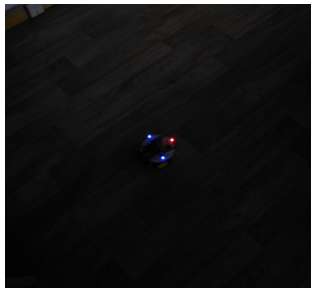Figure 1. Dark room; reduced light sensitivity

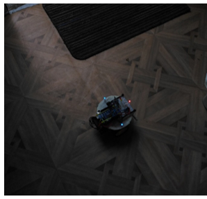Figure 2. Light room; reduced light sensitivity

The LEDs’ light now can be easily extracted even if the robot is in a brighter environment. However they are seen as little blobs and the light reflected by highly specular objects could be still present as noise, thus presupposing algorithm confusion and failure.

3) Camera focus

Most cameras support different focus modes, which helps the user adjust the focus:

• Auto-focus: automatically finds the best focus range, where most of the objects are sharp;
• Infinity: the focus is set to the farthest range leaving close objects dull;
• Macro: the focus is set to the closest range making nearby objects look sharp;
• Manual: leaves focus range to be adjusted manually be the user.

Figure 3 is taken with ISO 50, EV -2 and Macro focus in a bright environment. It appears, that reducing the camera focus not only blurs / removes noise from strong reflections, but also improves the LEDs light enlarging and saturating their blobs.

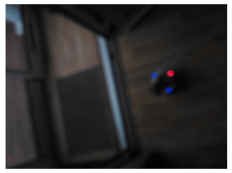Figure 3. Lighter room; defocused with reduced light sensitivity

4) Image analysis

So marking the robot with LEDs and adjusting the camera settings ensures more or less the same picture format with clearly expressed form of the robot regardless of the environment’s illumination. The taken pictures are analyzed with a computer vision algorithm. The taken approach relies on the following two color ranges:

1. a) RGB

Red-green-blue color model is an additive color model consisting of red, green and blue lights which combined give a wide range of different colors. This model is the base of the color space and is considered as the most identical and the easiest to understand by the human eye. Identical values of the three lights give a shade of the gray color. Keeping up the lights (at least one) gives a bright color while if all three of them are low will result in a dark color, close to the black one. In electronic devices a color in that space is represented by 3 Bytes – a Byte for the value of each light. Could be graphically represented by a cube (Figure 4a).

1. b) HSV

Hue-saturation-value is another range based on the RGB model. It is considered to be more convenient for usage in computer graphics and image editing. Hue represents the color intensity, saturation – the color completeness and the value is often call the brightness of the color. This color space is one of the most common cylindrical representation of the RGB model. Like the RGB color space a color of this space can be also stored in 3 Bytes – one for each channel (Figure 4b).

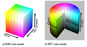Figure 4. Color model

The goal is to extract the blue LEDs for example. First an image representing the blue channel from the RGB color space is obtained (Figure 5).

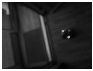Figure 5. RGB Blue channel

The image is greyscale because it has only a single channel. The blue blobs can be easily noticed, because they are colored in high grey value. But so does the door’s threshold. In fact every whiter object from the original image will have a high grey value in the blue channel image, because the white color in the RGB color space consists of high values in all of the three channels – red, green, blue.

The difference between the blue LEDs and the door’s threshold is obvious – LEDs are more colorful in the input image. A good representation of the color intensities is the saturation channel form the HSV color variant of the input image (Figure 6).

Figure 6. HSV Saturation channel

The difference is increased. The values of the LEDs are much higher than the one of the door’s threshold. The saturation image could be a perfect mask for ignoring white objects in all of the three channels from the RGB color space.

Next a masking of the blue channel is performed with the saturation image – applying a logical AND between the images’ binary data (Figure 7).

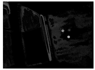Figure 7. Merged blue and saturation (blue_sat) channels

1. c) Binary image

Binary images are simple images whose pixels can have only two possible states – 0/1 or black/white. In most cases white pixels are considered as part of an object or of the foreground of the image and black – as the background. In computer vision binary images are mostly used as a result of different processing operations such as segmentation, thresholding, and dithering.

1. d) Image segmentation

Image segmentation is a technique to divide a digital image into multiple zones. The purpose is to detect objects and boundaries within the image.

1. e) Thresholding

Thresholding is one of the simplest image segmentation methods. It basically separate a greyscale image into a background and foreground areas as a resulting binary image. The algorithm is simple – if a pixel value is higher than a given constant (called threshold), it is classified as a part of the foreground regions and its value is set to 1 in the binary image. Otherwise the pixel is considered as a background one and a 0 is assigned to its value. The most challenging task while using this method is determination of a correct threshold value. Often a technique called Otsu’s method is used to solve this task. It calculates optimal threshold value by finding the minimal intra class variance between two class of points – one with lower values and one with higher values.

These image processing techniques are used by the LEDs recognition algorithm. After masking white regions in the blue image, a binarization is required. After the filtering a lot of dark regions have occurred. For certain LEDs’ pixel values are highest. Histogram analysis must be done only in the upper half of the histogram.

This is the extracted upper half of the merged image. Almost every time the LEDs’ pixel values are represented by the first highest peak. Otsu’s method is used over this part of the histogram. The calculated threshold is colored in green (Figure 8).

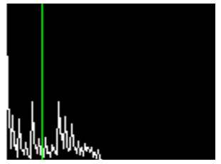Figure 8. Blue_sat histogram

This binary image is a result of thresholding and consequential dilation. With the use of connected-component labeling technique regions could be easily extracted and their centroids could be computed by the average point formula. These centroids represent the {x, y} coordinates of the blue LEDs (Figure 9).

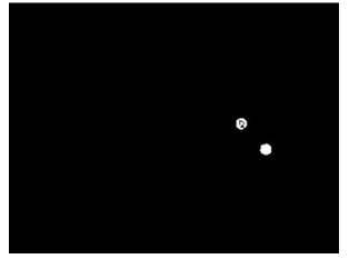Figure 9. Blue_sat binary image

The same algorithm could be applied for the other two RGB channels. Since there are no green LEDs results will be shown only for the red channel (Figure 10, Figure 11).

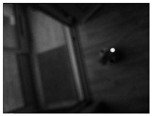Figure 10. RGB red channel

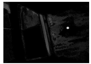Figure 11. Merged red and saturation (red_sat) channels

At the end {x, y} coordinates of the red and blue LEDs are present which makes the task of recognizing the robot completed.

2.3.  Transformation of 2D coordinates to 3D

The camera of the device shoots the robot’s sensors. The coordinates of the robot are calculated and sent to the robot using the Bluetooth interface. This process is presented at Figure 12.

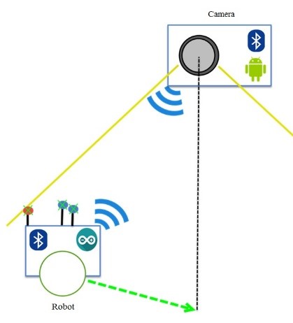Figure 12. Sending coordinates to the robot

The robot moving to the goal consists of turning and moving forward. Turning uses the angle between the direction of the robot and the goal direction. The LEDs coordinates, extracted from the image by the recognition algorithm, put in a Cartesian coordinate system result in the following model (Figure 13):

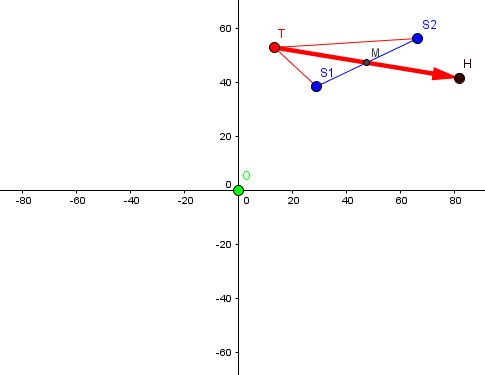Figure 13. Extracted LEDs coordinates in Cartesian coordinate system

The model is an approximate example. For increasing the detail in the interest area future models will be limited only to the first quadrant.

The turning phase should result in  pointing at O.

The environment in which the robot and the camera exist is three dimensional. Two dimensional object representations in such 3D world exist in so called planes. The camera takes 2D images which belongs to a plane determined by the camera. The robot on the other hand is a 3D object. Its representation in the 2D image is a projection of itself in that plane. Robot’s LEDs are attached in a way that keeps them on equal distance from the floor. It could be assumed that they are laying in a 2D plane parallel of the ground plane. What appears is that the extracted coordinates of the LEDs are their projections on the phone’s plane, moreover the center of the image is a projection of the robot’s target.

The following task arises: determine the robot’s position and orientation against its target by the given projections’ coordinates. After little mathematical analysis it appears that these coordinates are not enough for solving that given task. But that is not all. The robot knows the position of its LED sensors (Figure 14).

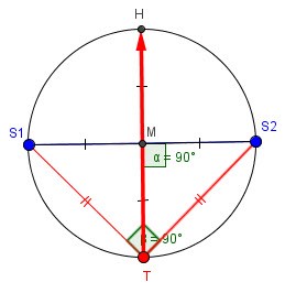Figure 14. Robot representation in its plane

The symbols in the diagram have the following meaning:

• T – tail point, representing the red LED with the extracted coordinates,
• S1, S2 – side points, representing the blue LEDs with the extracted coordinates,
• – the center of the image/coordinate system, representing the goal’s position,
• M – midpoint of the S1S2 segment, representing the center of the robot around which the robot should turn
• H – the T’s mirror point against M, representing the head of the robot,
• – a vector indicating robot’s size and the direction it is looking at.

This model is representation of the robot in its plane. It knows where are its head, center and tail, what size is its diameter and that the LEDs form an isosceles right triangle. All that is left to be found is the target’s coordinate against the robot in that plane – the O point. After that the value of the turn angle is defined by the points H, M, O. The distance to O is defined by (2):

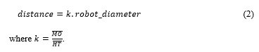Since the robot knows its physical diameter and the distance depends on a proportional variable the robot’s plane doesn’t need to be the same size – just the same proportions.

2.4.  Analytic Geometry for Transformation

The technique for accomplishing the task is simple and relies on basic laws from the Analytic geometry. Analytic geometry studies geometry using coordinate system – mostly the Cartesian one to deal with equations for planes, lines, points and shapes in both two and three dimensions. It defines, represents and operates with geometrical shapes using numerical information.

The current algorithm operates only with 2D coordinates {x,y} and the following shapes are being used:

Point

Represented by one pair of {x, y} coordinates which defines its position on the coordinate system.

Angle

Represented by single real value in radians or in degrees in the intervals respectively [0, 2π) or (-π, π] and [0, 360) or (-180, 180].

Line

Represents an unlimited straight ray. It is defined by (2):

the tangent of the angle between  and the line; it has a constant value,

the offset between the intersection of  and the line and the center point, it has a constant value.

Laws

The following laws are used by the algorithm:

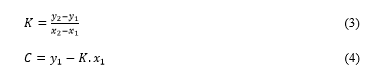
Line from two points p1 and p2 (3)(4)

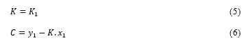
Line parallel to line  passing through point  (5)(6)

Intersection point of two lines  and  (7)(8)

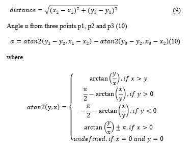
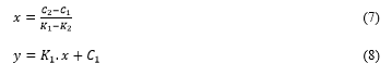Distance between two points p1 and p2 given by the Pythagorean theorem (9)

2.5.  Transformation Algorithm Definition

There are two planes – the phone’s one and the robot’s one, several laws, extracted points and real proportions. The two planes have to intersect somewhere in the space. If not that means they are parallel – the camera is parallel to the ground and the searched target’s position is in fact the center of camera image. But in most cases it is not and the two planes intersect. If the actual intersection line is found, distance from the camera to the robot could be computed. But since the result could be proportional that operation is unnecessary and the intersection line could be any line from the two planes. Of course the shapes need to keep original robot proportions. It is assumed that the intersection line is the one that passes through the two blue points giving the following model as a result (Figure 15).

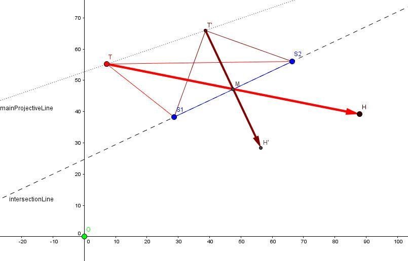Figure 15. Intersected planes with an example projection line

The dark color has shapes in the robot’s plane while brighter ones – in the image plane; a shape’s projection has the same name with suffix ’.

T’, H’ – projections of T and H, showing how would T and H coordinates be if the image’s plane was parallel to the robot’s one.

As it can been seen on Fig. 4 S1, S2 and T’ also define an isosceles right triangle in 2D – the proportions are kept.

A line could be defined from either T and T’ or H and H’ and could be called “main projective line”. All newly defined projective lines have to be parallel to this main one.

Let’s define the following shapes (Figure 16):

• Line from O and M called “center line”;
• Line from T and either called “side line” that can intersect the “center line”;

Intersection point SI from the center and side lines.

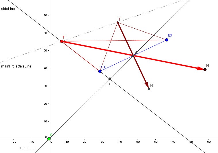Figure 16. Center line intersecting one of the side lines

The “side line” is defined using S1 which in this case is correct since the side line is not parallel to the center one. But there is a possibility that the line from T and S1 may not intersect the center line. If such case occurs the side line should be defined using S2. For certain T, S1, S2 form a triangle so if S1 is not appropriate for defining the side line, S2 will definitely be.

Next step consists of defining the following shapes (Figure 17):

• Side line’s projection – line from T and S1 (or S2 if S1 was not relevant during the previous step);
• Projection point of SI on the side line’s projection.

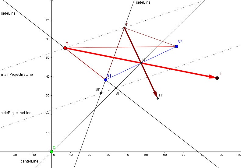Figure 17. Projecting the side intersection line

Defining a projection of a point on a line consists of two steps. Firstly a projective line must be defined. That line passes through the projected point and is parallel to the main projective line. The projection point is considered the intersection point of the projective line and the line that it is supposed to lie on. In this case the projected point is SI, the projective line is sideProjectiveLine and the projection point is SI’ that lies on sideLine’.

The final algorithm step consists of defining the following shapes (Figure 18):

• Define a line from M and SI’; since SI’ is a projection of SI along with the fact that SI and M lay on the center line, it could be stated that this new line is the projection of the center line;
• Define the projection of O on the center line’s projection.

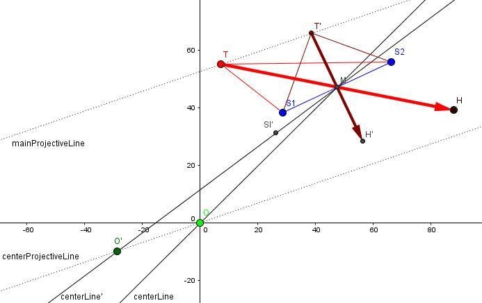Figure 18. Projecting the center line and center point

O’ is the projection of O which is defined the same way SI’ was. But this time the projective line is centerProjectiveLine and the second line for intersection is centerLine’.

O’ now represents the location of the target in the robot’s plane.

The result projection is shown on Figure 19.

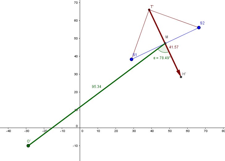Figure 19. Result of the plane transformation algorithm

Given that point the angle H’MO’ could be easily computed using the declared law.

The lengths of the segments MO’ and H’T’ are also known which enables the evaluation of (1):

3. System requirements and specification

3.1.  Mobile robot

The robot used in this project is based on the Arduino platform. It is an open-source microcontroller-based kit for building digital devices and interactive objects that could interact with the environment with sensors and actuators. Arduino board provides set of analog and digital I/O pins which enable connectivity with external physical devices. Programs for Arduino are written in either C, C++ or Processing.

3.2.  Arduino board

Robot’s controller board is an Arduino UNO R3, which is a basic microcontroller board, suitable for simple startup projects. It supports Universal Serial Bus (USB) with the help of which a serial communication could be established with PC and other devices and could also supply power to the board. Usually programs are built and compiled on a PC and further transferred to the board using the USB. It has also a 2.1mm center-positive power jack for external power supplies.

The board, used for assembling the robot, has the following parameters:

• Microcontroller: ATmega328
• CPU: 8-bit AVR
• Clock: 16MHz
• Memory of 23KB flash, 2KB SRAM and 1KB EEPROM
• 14 I/O pins
• 6 Analog Input pins
• Physical parameters: 68.6×53.4mm , 25g weight

3.3.  Robot body

For basic movements a simple 2 Wheel Drive (2WD) structure is used. This is a DIY 2WD double leveled plastic chassis. It consists of 2 wheels with separate gear motors, full-degree rotating caster wheel as a third strong point and two decks. The wheels are positioned almost in the center of the structure. Their rotation in opposite directions will result in the whole structure spinning over its center. The two decks are ideal for separating the mechanics from the electronics.

3.4.  Motor shield

The motor shield of the robot provides simple motor control. It provides a control of a motor’s speed, direction and braking along with sensing of the absorbed current. This board is stacked over the Arduino board.

3.5.  Bluetooth module

The robot is supplied with additional Bluetooth communication module.

3.6.  Magnetometer

HMC5883L is a Triple-axis Magnetometer (Compass) board. With the help of this sensor the robot can determine the direction it is facing. Furthermore using it the turning accuracy could be increased.

3.7. Camera

The project definition assumes that the robot establishes a communication with a remote device with a camera. It has one communication module – Bluetooth, therefore the remote device is required to have not only a camera but also Bluetooth communication technology.rduino board.

4. System Design

4.1.  General Design

Figure 20 gives an overview of the system’s design.

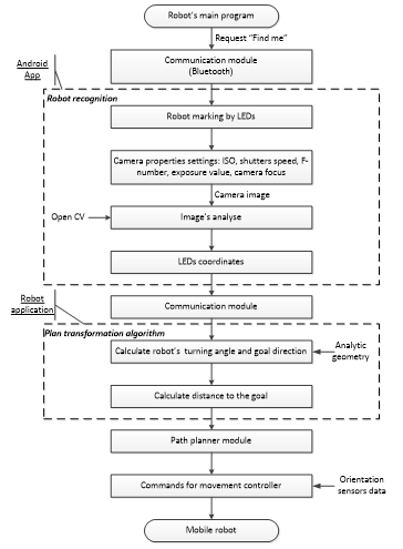Figure 20. Flowchart of the system’s general design

4.2.  Robot Software Design

The software for the robot is build based on the Arduino API keeping identical design to the general one.

The design is similar to the robot side of the general diagram. The difference is that the software is built over Arduino core API while the other is more abstract.

Abstract2WDController and Motor classes are meant to be an API to the Arduino Motor shield. They encapsulate pins reservation along with basic Arduino methods for setting different digital and analog levels to the pins.

• Motor – class, representing single motor channel of the Motor shield. It adjust its pins modes and levels using Arduino basic subroutines. Represents an API to the Motor module from the general diagram.
• Abstract2WDController – abstract class, encapsulating the declaration of two motor channels with the specific pin mapping for the Arduino Motor Shield. It also defines a basic interruptible motor control leaving the motors’ parameters to be adjusted by the class’ successors.
• Compass – an interface declaring a minimum behavior that one true compass object should implement.
• AngularController2 – an extension of the 2WDController providing forward movement and turning operations. In order to do accurate turns it uses a Compass object to determine its orientation. It has a predecessor sharing the same name and interface but not so successful. More information about them in the Implementation chapter.

The two controller classes could be considered as a representation of the Movement Controller module from the general diagram.

• ExSoftwareSerial – extends the Arduino’s SoftwareSerial library providing methods for reading not-string based data types from the upcoming stream. These methods support error handling and time-out periods. This class represents the API to the robot’s Communication module from the general diagram.
• TargetFinder – class implementing the main Plane transformation algorithm. It takes the {x,y} coordinates of the tail and the two side points and determines what turn has to be made in order to make the robot face the target and how far it is. This class does relates to the Path Planner module from the general diagram.
• Main – class representing the Main program. It binds the three features of the robot (communication, brain and motion control) together to complete the main goal of the project – staying in the center of the camera frame. This class delegates communication with the remote camera and controls the data flow from it through the TargetFinder to the Movement Controller.

4.3.  Camera Software Design

The software written for the remote camera is built based on the Android API but keeps its core identical to the general idea. Keeping the fact that the software is more or less a mobile application it has to have highly intractable user interface in order to monitor the system. The design extends the general one providing additional monitoring support using Android UI tools.

4.4.  Application Overall Design

This design shows how application’s modules are bound together.

• Bluetooth package – this package contains all defined Bluetooth classes. These classes are façades of the Android’s Bluetooth API and provides additional exception handling techniques and device discovery tools.
• Camera package – contains Camera classes extending the functionality of the Android’s Camera API. It implements different tools for serving the application’s specification. Camera preview class is present for handling each frame captured by the camera sensor. Additional Image processor is defined for analyzing images and a Custom camera class providing programmable interface to the project specific camera parameters for adjustment.
• Robot package – classes for handling robot requests. They implement features as robot communication managing, robot data translation and robot recognition.
• Graphical user interface (GUI) package – classes observing the core objects and updating the user interface when events occur
• Main Activity – manager class; creates all class hierarchy binding different modules together. It is responsible for resource acquiring and releasing such as Camera and Bluetooth hardware modules reserving, communicator and image processing threads handling on application starting and closing. It also appears as a controller to the main UI window granting classes form the GUI package an access to the UI objects.

4.5.  Core Design

The design, presenting the core of the application, does not differ much from the general one.

• Bluetooth classes – façades to the Android’s Bluetooth API; represent the interface to the device’s Bluetooth (the Communication module of the mobile device).
• BluetoothModule – manager class; creates BluetoothConnection objects, deals with the Bluetooth hardware’s settings and takes the responsibility of acquiring and releasing it along with closing all opened connections.
• BluetoothConnection – establishes bidirectional RF connection to a single remote device and is responsible for all data that flows in and out the device.
• RobotCommunicator – manager class; as the name suggests it completely implements the functions of the RobotCommunicator module from the general design. Additionally it uses the BluetoothModule to connect to the robot and a separate decoder called RobotTranslator to get a RobotRequestEvaluator object for handling the current request.
• RobotTranslator – factory for RobotRequestEvaluator objects; it takes the received request from the communicator and decides what evaluator to return.
• RobotRequestEvaluator – interface that unifies the type of all evaluators’ responses – a byte array as specified by the BluetoothConnection’s method “sendData”.
• CustomCamera – façade based on the Android’s Camera API providing interface to the Camera module and access to the following adjustable camera parameters (focus mode, ISO, Auto-exposure lock and exposure compensation)
• CustomCameraView – camera preview; implements frame handling that submits each new camera frame to the CameraImageProcessor and to a UI preview surface.
• CameraImageProcessor – singleton; fully implements the Image Analysis algorithm using external image processing native library – OpenCV; the result represents all extracted red and blue regions; represents the Image Processor module from the general design.
• Robot LED Image Recognizer – singleton; analyzes the extracted regions from the Camera Image Processor trying to recognize the robot. If successful, it converts the appropriate coordinates to a binary data. If the robot is not successfully detected from the current regions, modifications of the camera’s exposure are made and next result is awaited. Combinations of all available low exposure parameters are being tried.

4.6.  User Interface Design

The whole monitoring’s implementation is based on the Observer design pattern (Figure 21). It consists of objects called Observers that are listening for activity or changes in other objects called Subjects or Observables. Observer register to a Subject which hold a list with subscribed Observers. Each time a Subject do some activity or change state it notifies all its registered listeners providing them with the required information. Using this pattern constant looping (listening) in the listener classes is avoided.

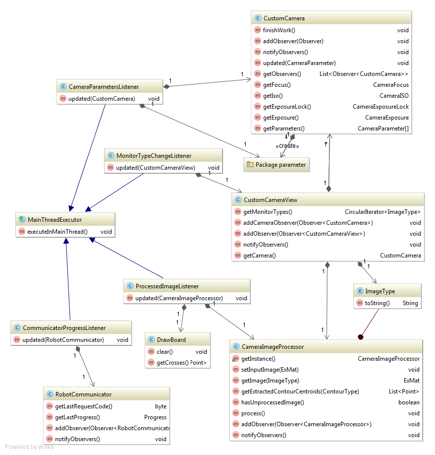Figure 21. UML class diagram of the Android application’s UI layer along with the observed core classes

• Main Thread Executor – it is an abstract class providing support for executing subroutines in the main thread. Android’s specification states that all interactions with user interface objects have to be done by the main thread also called UI thread. Also it highly recommends long-running tasks to be not executed by the main thread because it may result in UI freezing or lagging. Main Thread Executor is ideal for classes that mainly interact with the UI but are being accessed by objects running in separate threads – like the Robot Communicator or the Camera Image Processor.
• Communication Progress Listener – this class observes the Each time a communication activity is being done the communicator notifies its listeners. Interaction between the communicator and its observers is being done using Progress typed objects. The Communication Progress Listener updates an UI object each time new Progress object becomes present.
• Processed Image Listener – an observer of the When an image has been processed the processor updates its observers. The listener retrieves the extracted regions from the picture and displays them to the screen using a Draw Board. Draw Board is an which represents an Android UI Surface that is positioned above any else UI object in the main UI window. It implements functionality for drawing crosses.
• Monitor Type Change Listener – observes the Custom Camera View. By definition this custom view class handles all preview images from the Camera and sends them to both the Image processor and an UI preview class. Some additional monitoring was implemented giving the opportunity of displaying not only the original image but also intermediate processed image from the Image analysis algorithm. The Image processor provides access to such images via Image Type Clicking the view changes the type of the send image to the UI preview. The Monitor Type Change Listener is notified in case of such events and reflects the displayed image type’s string representation to a UI textbox.
• Camera Parameters Listener – Camera observer; the Robot recognition technique requires camera hardware adjustments. In this application camera parameters are being changed dynamically. Camera Parameters Listener outputs the customizable parameters to the screen and is being notified each time a change occurs.

Figure 22 demonstrates the common work of the application.

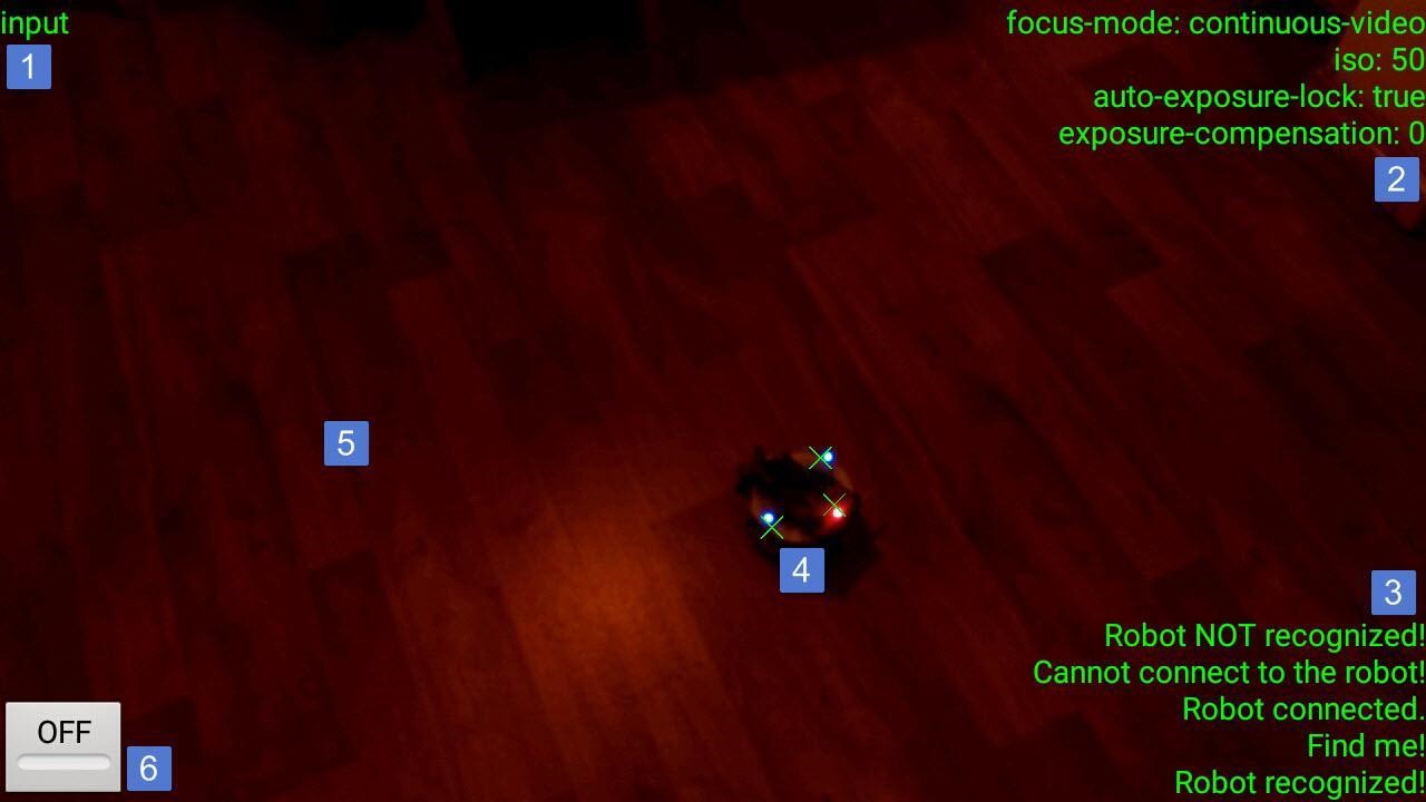Figure 22. Screenshot of the Android application with marked UI objects

The number markers has the following meaning:

• This is a text label that is being handled by the Monitor Type Change Listener. It displays the preview image’s type.
• A multiline not-editable text area. It is modified by the Camera Parameters Listener each time a camera parameter is changed. Presents the current camera’s settings.
• Another multiline area that keeps track of the Robot Communicator‘s progress. It is being handled by the Communication Progress Listener.
• Crosses drawn by invoking Draw Board methods from the Processed Image Listener.
• Touching the screen will change the preview image. The new image’s type will be presented in the Label 1.
• It is a switch button that forces the Image Processor work even when robot communication is not present. Used for high-end monitoring but consumes more battery power.

5. Testing and Evaluation

5.1.  Android Application

1) Robot recognition algorithm

The application was tested on three devices with quite different hardware specification. The results are summarized in Table 1.

Table 1. Camera application test results

Device model	Android	CPU	Camera parameters	Remarks
Asus ZenFone 2 Laser	API 21 v5.0 Lollipop	Qualcomm Octa-core	Focus mode ISO Exposure	Smooth performance; Fast image analysis; Robot cannot be recognized while on bright surface
LG Optimus G	API 19 v4.4 KitKat	Qualcomm Quad-core	ISO Exposure	Smooth performance; Fast image analysis; Robot cannot be recognized while on bright surface or if some noise is present.
Sony Live	API 14 v4.0 Ice Cream	Qualcomm Single-core	Exposure	Smooth performance; Fast enough image analysis; Robot cannot be recognized at all.

The following conclusions are summarized:

• The presence of several background threads doesn’t badly affect overall performance on a Qualcomm CPU with less cores;
• Automatic or not-present ISO setting is not recommended;
• Support of a close focus range could ignore noise;
• The recognition depends on the supported editable camera settings. An advanced intelligent robot recognition algorith is needed to remove this dependency.

2) Application Stability

After a lot of testing and debugging it could be stated that OpenCV’s matrix object Mat is not being automatically released on garbage collection as defined in the library’s documentation. Therefore it should be programmatically released before dereferenced. Otherwise a memory leak occurs which could cause system’s instability.

5.2.  Robot behavior

1) Plane transformation algorithm

The plane transformation algorithm is tested with different coordinates of the LED sensors, i.e. with three input data into a Cartesian coordinate system with range [-5; -5] ÷ [5; 5].

For resolution 2 of the value of coordinates 6 values per a coordinate are possible: -5, -3, -1, 1, 3, 5. Three input points have two coordinates with 6⁶ = 46656 test cases (Table 2).

Table 2. Results from test 1

Experiments	Number of tests	Percent	Conclusion
Total	46656	100%
Passed	36524	78.28%
Exceptions	10132	21.72
·          Handled	6048	12.96%	The three points lay on one line or two of them overlap.
·          Not handled	4048	8.75%	To be analyzed in future.

The tests from resolution 1 are presented in Table 3:

• each coordinate has 11 possible values in range [-5; 5];
• test cases: 116 = 1 771 561 possible combinations.

Table 3. Results From Test 2

Experiments	Number of tests	Percent	Conclusion
Total	1 771 561	100%	Conclusion
Passed	1 613 506	91.08%
Exceptions	158 055	8.92%
·          Handled	84 473	4.77%	The three points lay on one line or two of them overlap.
·          Not handled	73 582	4.15%	Further analysis

More combinations lead to less chance for an exception. Even a camera with low quality can take images with resolution of 1MP. This means, that the number of combinations is great and the occurrence of exceptions is practically not possible.

2) Turning accuracy

After continuous manual testing an anomaly has been discovered. The magnetometer (compass) sensor does not always gives adequate data and thus resulting in Movement controller’s confusion effecting the turning accuracy. The sensor has been tested in separate project with all magnetic components (motors, battery) detached from the robot but the problem still occurs. The issue could be caused by hardware defect but another module is not available at this state.

6. Conclusions and Future Work

The results from the experimental tests prove that the system is stable and effective with different devices and resolutions of the camera. This means, that a mobile robot, equipped with a usual camera, could be practically exploited for solving tasks as moving through dangerous spaces, searching for victims of disaster events, etc.

The future work will be directed to implementation of intelligent software controller, using neural network for detection and recognition of the robot image. More advanced orientation sensors (accelerometer, gyroscope) will be integrated and robot’s physical parameters (wheel diameter, motor RPM, robot size) will be used by the algorithm.

Conflict of Interest

The authors declare no conflict of interest.

1. M. Karova, I. Penev, M. Todorova, and D. Zhelyazkov, “Plane Transformation Algorithm for a Robot Self-Detection”, Proceedings of Computing Conference 2017, 18-20 July 2017, London, UK, ISBN (IEEE XPLORE): 978-1-5090-5443-5, ISBN (USB): 978-1-5090-5442-8, IEEE, 2017.
2.  C. Connolly, J. Burns, and R. Weiss, “Path planning using Laplace’s Equation”, IEEE Int. Conf. on Robotics and Automation, pp. 2101-2106, 1990.
3.  D. Lima, C. Tinoco, J. Viedman, and G. Oliveira, “Coordination, Synchronization and Localization Investigations in a Parallel Intelligent Robot Cellular Automata Model that Performs Foraging Task”, Proceedings of the 9th International Conference on Agents and Artificial Intelligence – Vol. 2: ICAART, pp. 355-363, 2017.
4.  J. Barraquand, and J. C. Latombe, “Robot motion planning: A distributed representation approach”, Int. J. of Robotics Research, Vol. 10, pp. 628-649, 1991.
5.  O. Cliff, R. Fitch, S. Sukkarieh, D. Saunders, and R. Heinsohn, “Online Localization of Radio-Tagged Wildlife with an Autonomous Aerial Robot System”, Proceedings of Robotics: Science and Systems, 2015.
6.  S. Saeedi, M. Trentini, M. Seto, and H. Li, “Multiple-Robot Simultaneous Localization and Mapping: A Review”, Journal of Field Robotics 33.1, pp. 3-46, 2016.
7.  T. Kuno, H. Sugiura, and N. Matoba, “A new automatic exposure system for digital still cameras”, Consumer Electronics, IEEE Transactions on 44.1, pp.192-199, 1998.
8.  T. Sebastian, D. Fox, W. Burgard, and F. Delaert, “Robust Monte Carlo localization for mobile robots”, Artificial Intelligence, Vol. 128, Iss. 1-2, pp. 99-141, 2001.
9.  W. Yunfeng, and G. S. Chirikjian, “A new potential field method for robot path planning”, IEEE, DOI: 10.1109/ROBOT.2000.844727, San Francisco, CA, USA, 2000.
10.  D. Hahnel, W. Burgard, D. Fox, K. Fishkin, and M. Philipose, “Mapping and localization with RFID technology”, Proc. IEEE Int. Conf. Robot. Autom., vol. 1, pp. 1015-1020, 2004.
11.  J. Flores, S. Srikant, B. Sareen, and A. Vagga, “Performance of RFID tags in near and far field”, Proc. IEEE Int. Conf. Pers. Wireless Commun., pp. 353-357, 2005.
12.  D. Lima, and G. de Oliveira, ”A cellular automata ant memory model of foraging in a swarm of robots.”, Applied Mathematical Modelling 47, pp. 551-572, 2017.
13.  B. Siciliano, and O. Khatib, Handbook of Robotics, Ed. 2, ISBN: 978-3-319-32550-7, Springer –Verlag, Berlin, Heidelberg, 2016.
14.  J. Shi, and J. Malik, “Normalized cuts and image segmentation”, Pattern Analysis and Machine Intelligence, IEEE Transactions on 22.8, pp. 888-905, 2000.
15.  R. Stengel, “Robot Arm Transformations, Path Planning, and Trajectories”, Robotics and Intelligent Systems, MAE 345, Princeton University, 2015.
16.  S. Se, D. Lowe, and Jim Little, “Mobile Robot Localization and Mapping with Uncertainty using Scale-Invariant Visual Landmarks”, The International Journal of Robotics Research, Vol 21, Iss. 8, pp. 735 – 758, 2002.
17.  T. Kuno, H. Sugiura, and N. Matoba, “A new automatic exposure system for digital still cameras”, Consumer Electronics, IEEE Transactions on 44.1, pp.192-199, 1998.
18.  D. Hahnel, W. Burgard, and S. Thrun, ”Learning compact 3D models of indoor and outdoor environments with a mobile robot”, Robotics and Autonomous Systems, Vol. 44, Iss. 1, 2003.
19.  L. Lee, R Romano, and G Stein, “Introduction to the special section on video surveillance”, IEEE Transactions on Pattern Analysis and Machine Intelligence 8, pp. 740-745, 2000.
20.  M. Beetz, “Plan-Based Control of Robotic Agents: Improving the Capabilities of Autonomous Robots”, ISSN-0302-9743, Springer-Verlag, Berlin, Heidelberg, New York, 2002.
21.  C. Richter, S. Jentzsch, R. Hostettler, J. Garrido, E. Ros, A. Knoll, F. Rohrbein, P. van der Smagt, and J. Conradt, “Musculoskeletal robots: scalability in neural control”, IEEE Robotics & Automation Magazine, Vol. 23, Iss. 4, pp. 128-137, 2016.
22.  D. Lima, and G. de Oliveira, ”A cellular automata ant memory model of foraging in a swarm of robots.”, Applied Mathematical Modelling 47, pp. 551-572, 2017.
23.  M. Alkilabi, A. Narayan, and E. Tuci, ”Cooperative object transport with a swarm of e-puck robots: robustness and scalability of evolved collective strategies”, Swarm Intelligence, Vol. 11, Iss. 3-4, pp. 185-209, 2017.

(Click Here)

(Click Here)