1. Introduction

The goal of this work is to extend the life of legacy Dexterous Social (MDS) robot [2]. This research-grade robots that have high quality electro-mechanical hard- robot originally debuted in 2008. The physical robot

ware by allowing them to make use of modern day hardware was custom built to support human-robot inrobotics software frameworks such as the Robot Op- teraction research. This includes the two 6-DOF arms erating System (ROS) [1], while keeping compatibility each with a 7-DOF hand. Each hand has four under-

with their existing calibration and monitoring tools. actuated fingers. The robot also includes a 4-DOF neck The significance and the novelty of this work is in its and a 17-DOF face. All of the latter items enable differfocus on the compatibility with legacy robotic systems ent facial expressions, physical gestures, and grasping via the use of a lightweight middleware, a non-head- within a single robotic platform. of-line blocking buffer design, and real-time network daemon. This document details our efforts in creat-Given the goals of this work, our system must meet

Table 1: Summary of existing software robotic frameworks [4]

Framework	Concurrency Model	Data Sharing	Focus
ROS [1]	Processes	Proprietary TCP	Mobile Robots, Vision, and AI
ROS 2.0 [3]	Processes	Selectable DDS	ROS 1.0 + Real-Time Control
OpenRDK [4]	Threads	Shared memory, Proprietary TCP/UDP	Mobile Robots
Player [5]	Threads	Client/Server over TCP	Mobile Robots
YARP [6]	Processes	shared memory, proprietary TCP	Mobile & Serial Kinematic Chain Robots
MARIE [7]	Processes	Many (3rd Party)	Connecting Different Frameworks
OpenRTM-aist [8]	Threads	CORBA	General Robotics
Orca [9]	Processes	ICE[10]	Mobile Robots
JAUS [11]	Processes	Proprietary TCP/UDP	Standardization, Unmanned Systems
x-Ach [12]	Processes	Shared Memory, Proprietary TCP/UDP	Real-time Robotics

specific requirements. Firstly, the well-tuned and refined calibration procedures that are extensively documented for the robot must remain unchanged while extending the robot’s capabilities. Similarly, existing monitoring tools must remain functional, but often cannot be modified. Furthermore, with robotics and Artificial Intelligence (AI) research back in the spotlight and becoming more mainstream in recent years, a robot system must implement additional safety controls to allow researchers with no mechanical or electrical engineering background to use the robot while keeping the risk of damage to the physical system low. The system must also be capable of working securely over a network. Finally, the system must not be confined to a single programming language, allowing the user to use “the right tool for the right job.”

To keep compatibility with the legacy software, direct control is implemented by commanding the MDS Robot over the Controller Area Network (CAN) bus via a dedicated real-time daemon. A process based controller approach is used for the control system using a “first-in-last-out” (FILO) non-head-of-line blocking ring buffer type of shared memory. This allows for the use of multiple programming languages in the same system. This also gives each controller the ability to read the newest data first which is typically of most importance to real-world robot controllers. SSH tunneling is used when secure connections between network connected controllers is required. Real-time collision avoidance with a robust inverse kinematics solution is implemented within the MDS-Ach system allowing for a multitude of types of users to safely control the robot. In the following sections, we describe our methodology and provide usage examples of the system. We also include, in the appendix, a description of the tools and the implemented API. Please note that this paper is heavily based on and is an addition to the authors previous work in Lofaro et. al. [13]. This work adds detailed instructions and examples of how to utilize the MDS-Ach system.

2. Background

There are currently many implementations of middleware for robot systems. The most notable one is the Robot Operating System which is commonly known as ROS[1]. ROS is a middle-ware which is TCP-based. It allows for communication between different controllers other over “topics.” This is typically done to connect the hardware systems of the robot such as the sensors and actuators to the logic and control. Its biggest strength is large ecosystem. Additionally, ROS is most useful for systems that require many controllers but do not require real-time capabilities. Currently ROS 2.0 [3] is being developed. ROS 2.0 will add real-time capability to the system. Because of the latter MDS-Ach is written specifically to be compatible with both ROS 1.0 and 2.0.

The YARP system, or Yet Another Robot Platform, is a C/C++ based middle-ware. The purpose of YARP is to connect control processes, sensors, and actuators. YARP is tested on Windows, Linux, and OSX [6]. It uses shared memory, over TCP when needed, for communication between the YARP server and clients. Nonblocking and latest data first reading is implemented via double and triple buffers. YARP is currently limited to a C/C++ API.

OpenRDK is an open source framework for robotics [4]. It uses socket communication and shared memory to implement its thread based architecture. This impressive control system utilized linking techniques and blackboard-based communication to allow for input/output data port conceptual system design. OpenRDK is a thread based design. Our desired system is processed based not thread based.

Joint Architecture for Unmanned Systems, also known as JAUS [11], was originally an initiative started in 1998 by the United States Department of Defense (DoD) to develop an open architecture for the domain of unmanned systems. JAUS was formerly known as Joint Architecture for Unmanned Ground Systems (JAUGS) and is built on five principles: vehicle platform independence, mission isolation, computer hardware independence, technology independence, and operator use independence. Still in use by the DoD, JAUS communicates with other systems over TCP and/or UDP. Though a formidable system, the public ecosystem is relatively small when compared to competitors. A comparison of the above-mentioned middleware, but also other robotic frameworks can be seen in Table 1.

The x-Ach system is based on the Ach IPC, or inter process communication [12]. Current implementation of x-Ach include Hubo-Ach [12] for the Hubo series of robots, Android-Ach for phones, Shoko-Ach [14] for the underwater legged robot AquaShoko, MDS-Ach (this work) for the MDS Robot, and more. The x-Ach system is lightweight with non-head-of-line blocking like OpenRDK, however it uses processes for each controller instead of threads. Like YARP, we use the idea of newest data first. Like OpenRDK, we use shared memory and offer a choice between TCP and UDP depending on need. x-Ach is compatible with multiple languages including C/C++, Python, Java, etc. ROS currently has the largest robot controller ecosystem, however it is not real-time; ROS 2.0 will be real-time when completed. To leverage ROS’ ecosystem, x-Ach is written to be compatible and easily integrated with either ROS versions.

3. Methodology

This section details the methodology and implementation of the MDS-Ach system and is based on our original paper [13].

3.1. Controller Area Network Communication

A key goal of this work is to keep compatibility with older robot’s legacy software and well-defined calibration procedures. In this case the specific robto in question is the MDS Robot. We created the MDS-Ach system to connect directly to the robot via the CAN (Controller Area Network) bus. This is the communications bus that is concurrently used to control each actuator on the MDS Robot and is also used with the legacy system, in this case the MDS Motion Server. The CAN bus is specifically designed designed for multiple devices/controllers to communicate over it. The latter allows all of the legacy software, utilities, and tools to run, monitor, and calibrate the robot while allowing for integration with the state of the art robotic software. The direct communicating via the CAN bus results in keeping compatibility with the original software and tools without having to modify, recompiled, or in any way adjust these tools in order for the MDS-Ach system to run.

3.2.  x-Ach

The x-Ach system has a process based architecture.

This means that it runs individual controllers as independent, synchronous and/or asynchronous, processes. Each process communicates with each other over the IPC called Ach which is a circular buffer and is non-head-of-line-blocking [12].

Ach was chosen because it is low-latency (key for real-time control) and has a first-in-last-out (FILO) buffer. This allows controllers to get the newest information first while retaining the ability of reading older information at a later time if needed. The latter is very important to real-time robotic systems. Packed cstructs are used for messages types in order to keep the system archatecture agnostic. This means that x-Ach controllers running on different platforms (i.e. x86, amd64, ARM, and other systems) can communicate with each other despite the different memory block sizes. It is important to note that all of the memory types are well defined within the packed c-struct. For example a (int32 t) is used instead of (int) to ensure data congruence between different architecture.

Controllers communicate with each other over Ach channels. Each controller has a standardized input channel called “reference” (ref), a standardized processed reference output channel called “processed reference” (p-ref), and a standardized output channel called ”state” (state). Details on the reference (ref) channels can be found in (Section 3.2.1) and details on the state (state) channel can be found in (Section 3.2.2).

3.2.1. Reference Channels

Each process based controller has two reference channels. One is a standardized input channel called “reference” (ref) and one is a standardized processed reference output channel called “processed reference” (pref) The latter two channels are where other controllers can write, or publish, to and read from, or subscribe to, respectively. It is important to note that the reference (ref) channel does not bind. This means that multiple controllers can write, or publish, simultaneously to the same reference channel. The controller will only use the most recent message received and only utilize the other older messages if it is specifically needed.

The process can synchronize its control loop to the incoming reference (ref) input or be asynchronous (i.e. free running). The latter is useful for use and development of synchronous and asynchronous controller systems and controllers. Both of the reference channels, the input reference (ref) and the process output reference (p-ref), are identical in structure.

As stated in Section 3.2, the reference channels consist of packed c-structs. The size of the structure is dependent on the number of degrees of freedom (DOF) of the robot of the given robot. The reference structure contains joint-space references (JS-ref) and work-space (Cartesian space) references (WS-ref) (see Figure 5). This is in the same structure to allow for less complexity in the controllers’ number and types of sources and sinks.

3.2.2.  State Channel

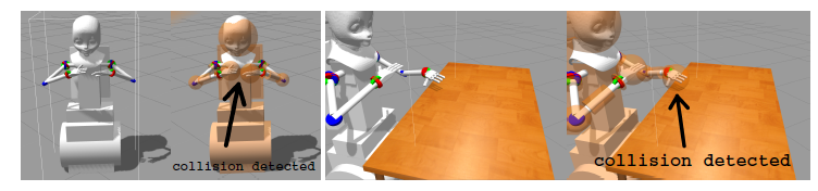Figure 2: High-resolution MDS Robot model (LEFT) next to the high-resolution MDS Robot model with the low-resolution collision models overlapped (CENTER LEFT). The collision models are simplifications of the high resolution geometry and are denoted in orange. The collision model is “over-sized” in order to help the system detect a collision before an impact actually occurs. Self Collision Avoidance Test: Robot does not collide when each hand is told to go to the same location. (RIGHT) World Collision Avoidance Test: Robot does not collide when the hand is commanded to a position that will collide with an object in its workspace.

Each MDS-Ach controller has one channel for the state what is real-only by other processes. Other controllers can read the most up to date state of the robot/controller by reading the state channel even if the given robot/controller is currently updating the state. For the implimentaiton on the MDS a daemon is created called the MDS-Ach daemon (see Section 3.3). This daemon publishes the most recent joint-space states including, but not limited to, actual position of the example the hand stops before it hits the table.

joint, last received reference/commanded position, joint load/current, etc. Like the reference channels the state channel is a packed c-struct. The size of the structure is dependent on the number of DOFs of the robot. An example use case for the state channel is the collision detection daemon in Section 3.4.2. This daemon reads the state channel and applies those values to its internal model to check for collisions in real-time. The daemon then outputs collision state of the robot on its state channel. This is done without disrupting the real-time performance of the MDS-Ach Daemon.

3.3. Daemon

The MDS-Ach daemon is the bridge between the CAN bus, which commands the MDS Robot, and the process based x-Ach controllers. The goal of all x-Ach daemons, in cluding the MDS-Ach daemon, is to be the “driver” for the given robot. The CAN bus is half-duplex running at a rate of 1.0 Mbps. Joint-space control and sensor feedback (i.e. reference and state information) is sent over the CAN bus to and from the daemon. The MDS-Daemon is specifically calibrated to keep the load on the CAN bus at approximately 60% of its bandwidth saturation. The latter is done to help guarantee real-time performance and on-time data delivery. The x-Ach daemons have been implemented and tested on multiple different types of robots with different CAN packet structures and a varying amount of communication buses. 200 hz real-time performance was achieved when utilizing multiple CAN buses (two) along with a specialized packet structure and the the utilization of the PREEMPT RT linux kernel [15] as seen in our previous work [12]. The MDS requires the use of only one CAN bus with a BAUD rate of 1Mbps and state-full packet structure. All of the latter limitations require us to run at 10 hz to guarantee real-time performance, with sub ms accuracy, for this specific robot.

The MDS-Ach daemon has an optional first-order real-time joint-space position smoothing filter. This filter is applied to the input from the reference (ref) channel (Section 3.2.1) before being applied to the control and sent to the robot over the CAN bus. The firstorder real-time joint-space position smoothing filter converges to within 95% of the reference input within 4.0 seconds and is enabled by default. This filter was added in order to reduce acceleration and jerk of each joint without limiting the maximum velocity.

The MDS-Ach daemon reads the reference command (as described in Section 3.2.1) in real-time and sends the command data over the CAN bus. This process is asynchronous in reference to the robot’s actuators control loop. If multiple commands are sent within one cycle only the newest one is read and processed. There is a zero order hold is there are no new commands between given control cycles. The except to this is during setup phases such as “homing”, resetting/error correcting, and other hardware setup/configuration specific commands. Additionally, during each cycle the MDS-Ach daemon requests and reads the information from the sensors via the CAN bus and writes it to the state channel (see Section 3.2.2).

3.4. Input Pipeline

The Main Controller receives the user-level commands in either joint-space or Cartesian-space, over the ACH shared memory. The latter input goes through the pipeline described in section below before it is sent to the Daemon (Section 3.3).

3.4.1       Joint Mux

The Joint Mux is an event-based process that takes in joint-space references from multiple processes. It updates the primary joint-space reference, which is sent to the MDS-Ach daemon, only with the joint-space references that are controlled by and updated by a given controller while preserving the ones that they controller does not have write permission to and/or were not modified. The MDS-Ach daemon is then sent the resulting consolidated (muxed) reference command. The purpose of this is to allows multiple controllers to update individual joints without conflicting with (overwriting) other joint commands while preserving a common message type.

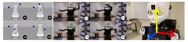Figure 3: Example of the MDS-Robot (MIDDLE) and its simulation (LEFT) utilizing the ik solver, joint smoother, and self-collision avoidance to move its hand in a square pattern while keeping all rotational degrees of freedom in the null space. (RIGHT) Coordinate system for the MDS Robot when using MDS-Ach.

3.4.2. Real-Time Collision Detection

The fully integrated real-time collision detection system utilizes the opensource simulator GazeboSim and ODE [16, 17] to ensure safe system operation. To guarantee the real-time performance, the system must detect self-collisions as well as collisions with objects in the environment within one time step of the MDS-Ach daemon (as defined in 3.3). To maintain compliance with the real-time deadline unneeded features of the simulator, such as physics, are disabled. This results in a reduced computational load. Additionally a geomet-

rically simplified/reduced model of the MDS robot is created. This model is comprised of basic shapes such as cylinders, boxes, and spheres. This simplified model is used to create the collision model to further reduce computational complexity and improve performance of the system. The performance improves because detecting collisions between two spheres only requires comparing the euclidean distance between the spheres centers and to the sum of the spheres’ radii. There is no collision as long as the sum of the radii is less than the euclidean distance from the centers. The same can be said for cylinders if the conditional measurement is made from the center of the sphere to the closest point on the axial line of the cylinder. Figure 2 shows the MDS Robot model with the collision model overlapped.

The collision state is written in state the message

format, as described in Section 3.2.2, to the Main Controller. If the reference position is free of collisions, a joint-space reference is sent to the the MDS-Ach daemon via the Joint Mux. The MDS-Ach daemon will execute the motion on the physical robot. If a collision is detected, the most recent safe joint-space reference values will be used for all the joints of the affected arm(s). “Expert” user is able to overwrite this behavior, if needed, by sending a joint-space command from the main controller.

3.4.3. Joint-Space Smoothing

When the robot is operating in situations where it is moving between joint-space configurations or required to stop its motion to avoid collision/self-collision (see Section 3.4.2), the safety of the robot’s joints needs to be ensured. Torque due to high joint-space acceleration is one of the primary causes of robot joint damage. We need to reduce the torque applied to the joints without causing joint-space overshoot. Furthermore this needs to be done in real-time and on-line. The motion at this level can not be pre-planned so it can be used in real-time tasks such as servoing or world interaction. This section shows how we reduce the acceleration, which reduces torque, on the joints while reducing the overshoot. The latter is done by applying the filter shown in (1).

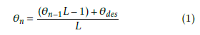Where θ_n is the output of the filter which is the new reference position (angle) the joint will be commanded to at step n; θ_n−₁ is the reference position to the joint from the previous time step, i.e. n−1; L is the weight of the filter (defined by its integer length); and θ_des is the desired reference position in joint-space that the joint is requested to go at time step n.

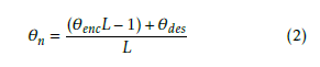
The position as recorded from the joints’ encoders

(θ_enc) are used to add joint-space compliance to the system. This is done by replacing θ_n−₁ in (1) with θ_enc as seen in (2). The use of the measured angle allows us to take advantage of the natural compliance in the system and magnify it. When the filter is applied it results in a pose “sag” due to gravity.

3.4.4. Inverse Kinematics

We utilize the “Inverse Jacobian” method for our online inverse kinematics solver. This is used to the joint-space angles for the commanded Cartesian-space (work-space) positions [18, 19]. The joint limits are utilized when constructing the the Jacobian during each cycle. During each step of the search the resulting pose is checked for self-collisions via ODE (see Section 3.4.2). A new intermediate goal position is created if a collision is found. The process is then repeated. The joint-space configurations found from the Jacobian IK is then passed through the filter discribed in (1) to prevent large steps in joint-space. Each step of the resulting filtered positions are then checked in real-time by the collision checker (Section 3.4.2) before being sent to the MDS-Ach daemon.

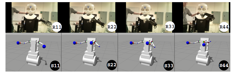Figure 4: Example of the MDS-Robot (TOP) and its simulation (BOTTOM) utilizing the IK solver, joint smoother, and self collision avoidance to move its hand in a box with the coordinates (x,y,z,θ_y) = (0.35m,0.45m,0.25m,null) → (0.35m,0.10m,−0.05m,null) → (0.45m,0.10m,−0.05m,null) → (0.45m,null,null,90^o) while keeping some linear and some rotational degrees of freedom in null space.

The Inverse Jacobian IK method is used because it allows control the required work-space degrees of freedom while the other degrees of freedom remain in null space. The MDS Robot is used for world interaction tasks such as opening doors (via pushing), grabbing cups, pushing buttons etc. thus having work-space degrees of freedom in null space is needed. In the door opening example (via pushing) the robot only degree of freedom that strictly matters is the x value (out of the robot’s chest – see Figure 3). The x value defines the distance the robot pushes the door open. The height (z) and the left/right distance (y) does not matter as much and thus can be left in null space. Furthermore the orientation (all three degrees of freedom) of the hand also belongs in the null space.

Solving for the required degrees of freedom for the given task, and leaving all the others in the null space, allows less iterations/computations for the solver resulting in a faster solving time and the ability to run in real-time. For MDS Robot, real-time constraints are satisfied if the joint-space values for a given Cartesianspace (joint-space) position are calculated in less than 0.5 sec. This is achieved when the desired Cartesianspace position can be described with DOF ≤4. The higher order of the required position requirements (i.e. the less degrees of freedom in the null space) the more time (on average) is required to solve the joint-space solution. A measured ∼ 0.7 sec is required to solve for a 5-DOF position and ∼ 1.3 sec for a 6-DOF on our contemporary computers using a single core. It is important to note that the latter calculated times are averages, also a solution is not guaranteed to be found even if one exists.

Figure 3 shows the MDS-Robot and its simulation utilizing the inverse kinematics daemon. The figure shows the MDS-Robot commanding its end-effector to move in a box pattern in real-time. A detailed description of the test can be found in Section 4.1.

MDS-Ach System Diagram

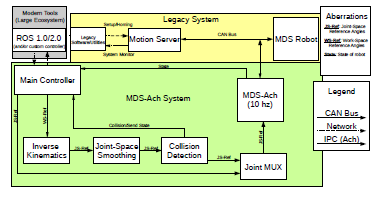Figure 5: MDS-Ach middleware: A real-time process based control system used to extend the research life of the MDS Robot.

3.4.5. Network Daemon

The network daemon utilizes achd, as a part of the Ach library, to share data over a “socket” supported network. The achd daemon pushes the state data from the primary control computer on the robot to the external “user-level” computer controller when new state data is available. When a reference command is updated by the user-level computer controller it is pushed to the primary control computer over the network by the achd daemon. Updates are only pushed or pulled when there is new state or reference data in order to conserve bandwidth. UDP is used by default for data transport to help facilitate tighter real-time performance. TCP or TCP over a SSH tunnel can be used by the user depending on timing, reliability, and security requirements.

More details can be found in our previous work [12].

3.4.6. Security

Intercepting and spoofing network traffic is a major threat to any robot system and the threat persists even on a properly configured Unix/Linux computer. These “man-in-the-middle” attacks allow a third party to control the robot using the existing controllers if they can spoof the feedback data [20]. To prevent a man-in-themiddle attack over the network, a secure SSH tunnel with pre-shared keys is used to transmit and receive state and reference data between the main controller and the user-level controller. Since SSH tunnel operates over TCP, the network throughput between the user-level controllers and the Main Controller is reduced, and may even affect the real-time performance.

3.5. External Framework Bridge

The ROS 1.0 and ROS 2.0 bridge allows us to make use of the extensive ROS ecosystem and serves as proof of concept for extensibility of this middleware. This bridge talks directly with the Main Controller via the Ach shared memory or the network daemon (3.4.5). This controller converts the state data published by the MDS-Ach system into ROS messages to be published again on specified ROS topics. To reduce latency (1) the state topic of ROS is synchronous with the state channel of MDS-Ach, and (2) the reference channel is synchronous with the state topic of ROS (seen Fig. 5).

4. Testing

At the conclusion of the MDS-Ach middleware development, we tested the software to confirm its functionality. We present the testing procedures and results of the inverse kinematics system (Section 4.1), the live self-collision detection system (Section 4.2), and the live external-collision detection system (Section 4.3).

4.1. Inverse Kinematics Test

To validate the usability of the inverse kinematics system, we performed couple tests to show its ability to move the end-effector to a position (4.1.1) and an orientation (4.1.2) in the Cartesian-space (work-space) while keeping other variables in the null-space. The coordinate system used for the IK tests is shown in Figure 3; the origin is the orthogonal projection of the base of the neck onto the line defined by the rotations points of the shoulders. x–y plane is horizontal. x–z plane extends in front and behind the robot while y–z plane extends to the sides. All signs of rotation follow the “right hand rule.”

4.1.1. Position Control IK Test

This section presents results showing that the endeffector can be moved between multiple linear Cartesian-space (work-space) locations (x,y,z) without constraining the end-effector orientation. The left arm is commanded and moved to the locations shown in (3) where S1, S2, S3, and S4 are the coordinates for the simulated robot and R1, R2, R3 and R4 are the coordinates for the real robot.

S1= R1=(0.40m,0.45m,0.25m)

S2= R2=(0.40m,−0.05m,0.25m)

(3)

S3= R3=(0.40m,−0.05m,−0.25m) S4= R4=(0.40m,0.45m,−0.25m)

The screenshots of the resulting motion can be found in Fig. 3.

4.1.2.  Orientation Control IK Test

This section presents results showing that the endeffector can be moved between multiple Cartesianspace poses (x,y,z,θ_y) while keeping the remaining orientations in the null space. The left arm is commanded and moved to the locations shown in (3) where S11, S22, S33, and S44 are the coordinates for the simulated robot and R11, R22, R33 and R44 are the coordinates for the real robot. In the case of the last motion (R44 and S44), θ_y is set to 90^o and a desired x to a value of 0.45m while all other degrees of freedom remain in the null space. The full set of coordinates for this test can be found in (4).

S11= R11=(0.35m,0.45m,0.25m,null)

S22= R22=(0.35m,0.10m,−0.05m,null)

(4)

S33= R33=(0.45m,0.10m,−0.05m,null) S44= R44=(0.45m,null,null,90^o)

This shows that the IK process can solve for some degrees of freedom while keeping the others in null space (see Figure 4). This improves system performance when higher fidelity solutions are not required for system operation.

4.2. Self-Collision Detection and Avoidance Test

To test the self-collision system as described in Section 3.4.2, we drove the hands to the same location using the IK system described in Section 3.4.4. Multiple instances of this test were performed. In all the runs, the hands stopped before colliding. Figure 2 shows one example of the multiple self-collision tests. In this instance of the test, both the left and the right hands were told to go to the (x,y,z) coordinates (0.3m,0.2m,0.0m). As expected, the hands did stop when the two parts of the collision model touched as shown in Fig. 2.

4.3. World-Collision Detection and Avoidance Test

To test the world-collision avoidance system described in 3.4.2, we drove the hand from the position stated in Section 4.2 out to an x value of 0.5m towards the table. We placed a model of a table in the simulated world where the real table would be. From there we drove the hand down in z. Similar to the results in 4.2 the hand would not move farther than the collision point between the collision model of the hand and the collision model of the table (see Figure 2). This was done for multiple objects and multiple collision locations.

5. Usage

This section documents how to start, stop, and use different MDS-Ach utilities. The MDS-Ach controls the MDS Robot via the CAN bus. It provides smoothing/filtering, multi-process control architecture, multilanguage support, inverse kinematics for right and left arm, and more.

5.1.Daemon Control: mds-ach

The MDS-Ach daemon is the process running the background that controls communications between the physical (or simulated) robot and the controllers. The daemon controls the CAN bus when connected to the physical robot. Section 5.1 describes the different input options and modes of the MDS-Ach daemon. A full description of the options for the console input for the MDS-Ach daemon can be found in Appendix A.

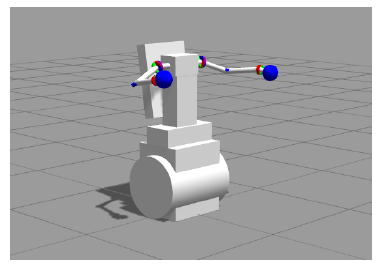Figure 6: MDS Robot simulated in Gazebo.

5.2. Startup Procedure

This section documents the startup procedure for the MDS-Ach system.

5.2.1. Initialize

We preserved the original MDS setup procedure provided by MDS manufacturer, Xitome. Once setup is complete, which include a fairly involved homing procedure for all the joints, the user is able to keep the Xitome subsystem running. User may not issue commands to any of the joints using the Xitome system once MDS-Ach is started.

5.2.2. Start Daemon

It is important that the MDS robot is in its homed configuration when starting the MDS-Ach system. This is because MDS-Ach system assumes the robot’s starting position to initialize the IK and the self-collision systems. If the robot is not in its “homed” position, than some joints will get a step input to go to the starting position. All starting positions are read from the anatomy.xml configuration file located in /etc/mdsach. This file is identical to that used by the Xitome system for configuration.

The MDS-Ach system can run on the robot (Option

1) and on a simulated robot (Option 2). Option 1 sends all of the commands over the CAN bus while Option 2 sends all commands to GazeboSim[16]. Both Option 1 and Option 2 have an x-Ach[13] abstraction layer between their respective communication buses and the controller. A full description of the implementation procedure can be found in Appendix B.

5.3. Examples

Examples of how to do basic operations using the MDSAch system on both the real robot and the simulator can be found in Appendix C. The examples show how to start the MDS-Ach daemon on the physical and simulated robot. An image of the simulated robot can be seen in Figure 6. All example code/software can be found in Lofaro et. al. [21].

6. Utilities

This section describes the utilities available for use with the MDS-Ach system. All utilities work seamlessly with the physical and simulated robot.

6.1. MDS-Ach Console

The MDS-Console utility allows the user to read and set individual joint angle values via the command-line. It also allows the user to read the Caretesian-space pose (6 DOF) of the end-effector and set the desired target pose (3, 4, 5, and 6 DOF). The console provides control interface for all the joints listed in Table 2. We included examples of single joint interactions, but also end-effector control, in Appendix D.

Table 2: Joint abbreviations (short and long) with definitions

Definition	< joint > (short option)	< joint > (long option)
Right Elbow Pitch	REP	RightElbowFlex
Right Shoulder Yaw	RSY	RightUpperArmRoll
Right Shoulder Roll	RSR	RightShoulderAbd
Right Shoulder Pitch	RSP	RightShoulderExt
Left Elbow Pitch	LEP	LeftElbowFlex
Left Shoulder Yaw	LSY	LeftUpperArmRoll
Left Shoulder Roll	LSR	LeftShoulderAbd
Left Shoulder Pitch	LSP	LeftShoulderExt
Right Wrist Roll	RWR	RightWristFlex
Right Wrist Yaw	RWY	RightWristRoll
Left Wrist Roll	LWR	LeftWristFlex
Left Wrist Yaw	LWY	LeftWristRoll
Torso Yaw	WST	TorsoPan
Neck Roll	NKR	HeadRoll
Neck Pitch (lower)	NKP1	HeadPitch
Neck Pitch (upper)	NKP2	NeckPitch
Neck Yaw	NKY	HeadPan

6.2. MDS-Ach Read

The MDS-Read utility allows the user to view the joint space references, state, and address of each active joint. This utility updates the information at ∼ 20Hz. It may be started or stopped at any time without affecting the overall system.

6.2.1. Prerequisites

Since MDS-Read is a monitoring tool, it must be started after the MDS-Ach is already running.

6.2.2. Startup

To start the MDS-Read utility, run the command below.

The expected terminal can be seen in Figure 7.

Bash/MDS-Ach Console:

$ mds−ach read

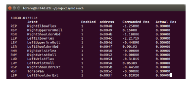Figure 7: Expected window for ($ mds-ach read)

• Note 1: If you are running with the simulator the state (Actual pos) will always be zero. When running on the physical robot the real position (in radians) will be shown.
• Note 2: If you make more joints “active” in the /etc/mds-ach/configs/mdsach.xml configuration file they will automatically show up in MDSRead.

6.3. Software Interface

The MDS-Ach system currently works with the C/C++ and Python programming languages. Appendix E describes the required libraries for each of the latter languages.

7. Operating in Joint-Space

This section documents how to use MDS-Ach to control the robot in joint-space. To move one, or multiple joint/joints the following steps must be followed:

• Open Ach Channels – This is the ring buffer shared memory that this controller communicates with MDS-Ach with.
• Create Required Data Structures – Standardized (packed) data structure that contains all of the reference and state data for the robot.
• Get Joint ID – Determine the IDs of the joint/joints to be controlled (See Table 2).
• Queue New Motor Position – Put the desired motor positions in the reference structure at the index position defined by the Joint IDs.
• Set Motor Position (put) – Write the reference structure that has been updated with the desired position for the desired joint to the reference Ach channel.
• Close Ach Channels on Exit – Though not required it is good practice to close the unused Ach channels upon exiting the controller.

Figure 8 shows the expected simulator window when following the above steps and setting the Left Elbow Pitch (LEP) and the Right Shoulder Pitch (RSP) to -0.2 rad and 0.1 rad respectively.

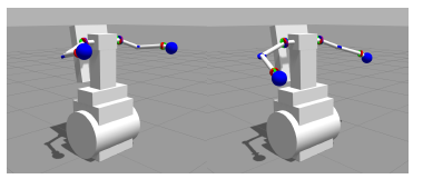Figure 8: Expected simulator window for ($ ./mdssimple-demo). (LEFT) Before running. (RIGHT) After running.

It is important to note that Appendix F is an depth explanation and example of how to setup the Ach channels for communication with the MDS-Ach system and how to control the robot in joint-space while using the smoothing filter process. Examples are given in C/C++ and Python.

8. Operating in Cartesian-Space

In this section we discuss end-effector operations in Cartesian-space which utilize forward and inverse kinematics controllers of the MDS robot.

8.1. Built-in IK Controller (Python)

The MDS-Ach system has a built-in inverse kinematics

(IK) controller for both the right and left arms. This controller automatically runs when the MDS-Ach system is started. The controller solves for one arm at a time.

The system begins to solve the IK equations automatically, when you post a new desired position on the IK reference channel. Below is a step by step of how you do this using Python.

8.1.1. Python imports

The following are required imports for the MDS-Ach system while using python: mds ach, ach, and mds. Other imports are for the given controller implementation.

Python:

import mds ach as mds import ach import time import sys import os import math

8.1.2. Create Open Ach Channel for IK

Ach channels are how you communicate with MDSAch. You simply write data to the channel and the robot can read the data in newest to oldest order. The section below shows you how to open an Ach channel. Please note that ach.Channel() takes a string as an input. Here we opened one channel. This is a different channel then found in previous sections because it is only for the IK controller.

Python:

# Open ACH Channel for IK k = ach . Channel (mds.MDS CHAN IK NAME)

8.1.3. Make IK Structure

Similar to controlling the robot in joint-space you need to set a reference structure to the desired work-space position. For this you need to initialize the structure. See below for the initialization of the work-space structure.

Python:

# Make new IK structure ikc = mds.MDS IK()

8.1.4. Setting the DOF controlled

When using the built-in IK controller you need to set the number of DOF that you are controlling. With this controller you are required to set the DOF in the following order: p_x,p_y,p_z,θ_x,θ_y,θ_z where p_n is the position on axis n and θ_n is the rotation about axis n. For example if you DOF is set to 4 you are controlling p_x,p_y,p_z, and θ_x. If you are controlling 2 you will control p_x and p_y. In the example below we are controlling 3, i.e. p_x,p_y, and p_z. This order can also be seen in Table 5.

Python:

# Set the amount of DOF you want to dof = 3

control

We set these to the values in Table 3.

Table 3: Inverse Kinematic Values Set for Example 8.1.4

Param #	Definition	Abbreviation	Value (rad)
1	Position in X	px	0.3
2	Position in Y	py	0.2
3	Position in Z	pz	0.0
4	Rotation in X	θx	Null Space
5	Rotation in Y	θy	Null Space
6	Rotation in Z	θz	Null Space

θ_x,θ_y, and θ_z are in the Null Space because we do

not care where they are as long as the first three parameters are met. We can set these values to what ever we want and they will be ignored. In this case we set them to zero.

Python:

# Set values for work−space in # [x , y , z , rx , ry , rz ] order eff = [0.3 , 0.2 , 0.0 , 0.0 , 0.0 ,

0.0]

8.1.5. Choosing Arm for IK

Here we pick the arm for the IK. Our options are set as enums in the mds ach.py and mds.h includes. All options for right and left arms can be found in Table 4.

Table 4: Definitions for left and right arms using mds ach.py in Python

Arm	Python Definition
Left	mds.LEFT
Right	mds.RIGHT

Here we set the arm to the left arm.

Python:

# set arm armi = mds.LEFT

8.1.6. Set IK Structure

Just as in the joint-space method, we need to the values in our structure before we send it to the robot. Here we set all of the parameters from above to the structure ikc that we created.

Python:

# Put setting into ik structure ikc .move = armi ikc .arm[ armi ] . ik method = dof ikc .arm[ armi ] . t x = eff [0] ikc .arm[ armi ] . t y = eff [1] ikc .arm[ armi ] . t z = eff [2] ikc .arm[ armi ] . r x = eff [3] ikc .arm[ armi ] . r y = eff [4] ikc .arm[ armi ] . r z = eff [5]

8.1.7.  Command the Robot

Just as with the joint-space controller you need to “put” the data on the ACH channel. Unlike the joint-space controller it will not move as soon as you send it. The controller will first have to solve the IK. Upon finding the solution the controller will send it to the robot. If a solution is found it will take anywhere between 0.1 and 5.0 seconds. If there is no solution found the robot will not move. Note: the robot limits its self to 1000 search iterations for an IK solution.

Python:

# put on              to ACH channel k . put ( ikc )

8.1.8. Running the Code

To run the code do the following within the mdsach/examples folder.

Bash:

$ python ms ik one . py

The expected terminal out can be seen in Figure 9.

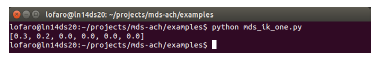Figure      9:         Expected      window     for     ($       pythonms ik one.py)

To check that the IK worked you can run the FK in the MDS-Ach console and/or run the simulator. The before and after of the MDS-Ach console is found in Figure 10 and Figure 11, respectively.

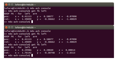Figure 10: Expected MDS-Ach Console window for (>> mds-ach-console$ get fk left). (TOP) Before running. (BOTTOM) After running.

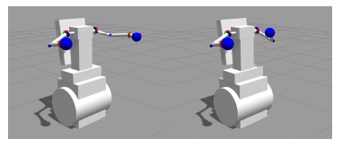Figure 11: Expected simulator window for ($ python mds ik one.py). (LEFT) Before running. (RIGHT) After running.

8.1.9. Full Code

The full example can be found below as well in the file: mds-ach/examples/mds_ik_one.py

8.2. Built-in IK Controller (C/C++)

The MDS-Ach system has a built-in inverse kinematics

(IK) controller for both the right and left arms. This controller automatically runs when the MDS-Ach system is started. The controller solves for one arm at a time.

The system works by starting to solve the IK equations when you post a new desired position on the IK reference channel. Appendix G has a step by step of how you do this using C/C++ which is identical in methodology to the Python implimentaiton in Section 8.1.

8.3. Making a Box using Inverse Kinematics (Python)

This section shows you how to control the MDS robot via the built in IK module. This example shows us using solving a 3 DOF IK. The method used can be expanded to any DOF between 1 and 6.

The example given is the robot moving its left hand in a 0.5 m box 0.4 m away from the origin. The hand will not move in the x plane, only in the y and z.

8.3.1. Making the Box

The following points will be hit in order: (0.4,0.45,0.25) → (0.4,−0.05,0.25) → (0.4,−0.05,−0.25) → (0.4,0.45,−0.25) with all units in meters. Example Python code for state flow. Note state 0 (0.3,0.2,0.0) is the initial state and will not be returned to.

Python:

if i i == 0: c = [0.3 , 0.2 , 0.0] i i = 1 elif i i == 1: c = [0.4 , 0.45 , 0.25] i i = i i +1 elif i i == 2: c = [0.4 , −0.05 , 0.25] i i = i i +1 elif i i == 3: c = [0.4 , −0.05 , −0.25] i i = i i +1 elif i i == 4: c = [0.4 , 0.45 , −0.25] i i    = 1

8.3.2. Select Arm

The following selects the arm used for the IK. You may use “left” or “right” for the left and right arms respectively.

Python:

arm = ’ l e f t ’ armi = −1 if arm ==             ’ l e f t ’ : armi = mds.LEFT if arm == ’ right ’ : armi = mds.RIGHT

8.3.3. Parse Desired Position

Parse the desired position for the end-effector to 6 DOF array.

Python:

dof = 3 eff = [0.0 , 0.0 , 0.0 , 0.0 , for i       in range (0 , dof ) : eff [ i ] = c [ i ]

0.0 ,

0.0]

8.3.4.  Set Desired Position

Sets the desired position for the end-effector. ikc.arm[].ik method is the number of DOF that you will be controlling. ikc.arm[].t * and ikc.arm[].r * is the desired position and rotation of the end effector respectively.

Python:

if       armi >= 0: ikc .move = armi ikc .arm[ armi ] . ik method = dof ikc .arm[ armi ] . t x = eff [0] ikc .arm[ armi ] . t y = eff [1] ikc .arm[ armi ] . t z = eff [2] ikc .arm[ armi ] . r x = eff [3] ikc .arm[ armi ] . r y = eff [4] ikc .arm[ armi ] . r z = eff [5]

8.3.5. Send Desired Position to be Solved

The following sends the desired position and ik method to the IK controller to attempt a solution.

Python:

k . put ( ikc )

8.3.6. Running the Code

To run the code do the following from within the mdsach/examples directory Bash:

$ python examples/mds ik box example . py

The expected terminal output can be seen in Figure 12.

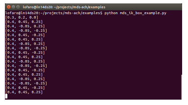Figure 12: Expected window for ($ python examples/mds ik box example.py). Time order is left to right, top to bottom.

The expected robot pose can be seen in Figure 13.

The latter figure shows the virtual robot not the physical robot.

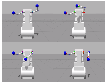Figure 13: Expected robot poses for ($ python examples/mds ik box example.py)

8.3.7 . Full Code

The full example can be found in the file: mds-ach/examples/mds_ik_box_example.py

8.4.  Inverse Kinimatics (IK) API

The Inverse Kinematic (IK) API utilizes the Inverse

Jacobian method to solve for the joint-space values given an end-effector position of each of the arms. The IK solver is capable of solving for any and all of the six degrees of freedom of the end-effector i.e. translation (x,y,x) and rotation (θ_x,θ_y,θ_z) while keeping the non-constrained position/rotations in Null space. The number of steps and error range can be specified by the user.

Appendix H gives an example of how to get and set the forward and inverse kinematics via the mds ik API. The goal of this tutorial is to solve for the joint-space values given the desired work-space values as found in Table 3.

9. Conclusion

In conclusion we have made a middleware called MDSAch that enables the legacy MDS Robot to be used with modern day robot software, thus extending its life as a research robot. Low-latency non-head-of-line blocking FILO shared memory and network connectivity is used to share data between real-time processes. SSH tunneling is used if a secure network connection between controllers is required. Built-in collision avoidance, inverse kinematics, and support for multiple programming languages was implemented to expand usability to our non-hardware-focused partners. Finally, a ROS interface was developed with specific focus on making it ROS 2.0 compatible to enable the use of the extensive ROS ecosystem. These combined contributions allowed MDS-Ach to significantly extend the research life of the MDS Robot.

Acknowledgment

This work was performed in part at the Naval Research Laboratory under the project Adaptive Real-Time Algorithms for Multiagent Cooperation in Adversarial Environments. The views, positions and conclusions expressed herein reflect only the authors opinions and expressly do not reflect those of the Naval Research Laboratory, nor those of the Office of Naval Research.

10. APPENDIX A Daemon Console

This section shows the specific console inputs available for the MDSAch system.

Console Input: $ mds-ach – Shows command options Console Input: $ mds-ach start – Start all channels and processes and console

• (no-arg) : Starts MDS-Ach system on CAN Bus 0 “CAN0”
• nocan : Starts MDS-Ach system with no output to real CAN Bus. Will output to the virtual can “VCAN42” instead

Console Input: $ mds-ach console – Starts the human interface console for MDS-Ach

Console Input: $ mds-ach stop – Close all channels and processes

Console Input: $ mds-ach make – makes all the MDS channels

Console Input: $ mds-ach kill – Emergency kill the daemon process Console Input: $ mds-ach killall – Emergency kill the daemon process and removes all ACH channels

Console Input: $ mds-ach resetbus – Resets the Bus Console Input: $ mds-ach remote – Starts a remote connection to xxx.xxx.xxx.xxx via achd

Console Input: $ mds-ach sim – Starts the sim in gazebo

• (no-arg) : Starts the sim in gazebo
• kill : Kills gazebo sim

Console Input: $ mds-ach changerobot – Changes the robot’s configuration file/anatomy

• (no-arg) : No Change
• isaac : Changes to Isaac’s anatomy
• lucas : Changes to Lucas’ anatomy
• octavia : Changes to Octavia’s anatomy

B Startup Procedure

To start the MDS-Ach daemon select one of the two options. Note: Both Option 1 and Option 2 will start the following processes:

• mds-daemon : primary control for the MDS robot
• mds-filter : filtering process to allow for step inputs
• mds ik module (python) : inverse kinematics (ik) controller for the MDS
  • (Option 1) With physical MDS robot:

Bash:

$ mds−ach       start

• (Option 2) With virtual MDS robot:

Bash (Start with no CAN Bus):

$ mds−ach       start     nocan

Bash (Start Simulator):

$ mds−ach sim

The simulator can be run with either (Option 1) or (Option 2) above.

C Examples

The following are examples of how to do basic operations using the MDS-Ach system on both the real robot and the simulator.

Run MDS-Ach Daemon:

Bash:

$ mds−ach       start

The resulting terminal windows should look like Figure 14.

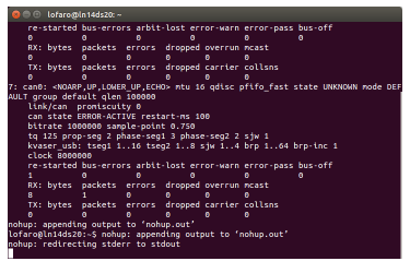Figure 14: Expected window for ($ mds-ach start)

Run MDS-Ach Daemon with simulator only:

Bash:

$ mds−ach       start     nocan

This command will start the MDS-Ach daemon. This should be run on the computer where the simulator is located. The MDS-Ach daemon (mds-daemon) will run in the background even if the terminal session is closed. This will run with the simulator and not with the real robot. Use this mode if you only want to use the simulator.

The resulting terminal windows should look like Figure 15.

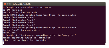Figure 15: Expected window for ($ mds-ach start nocan)

Run MDS-Ach simulator:

Bash:

$ mds−ach sim

Once the MDS-Ach Daemon is started (see above) you can run the simulator. The simulator is open loop in the respect that it does not feed back information to the MDS-Ach system. It is used as a visual representation of the robot for debugging and initial controller testing.

The resulting terminal windows should look like Figure 16.

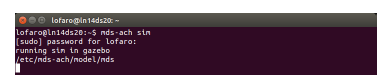Figure 16: Expected window for ($ mds-ach sim)

The resulting simulator windows should look like Figure 6.

D  MDS-Ach Console

The MDS-Console utility allows the user to get and set joint space values via the command line. It also allows the user to get the work-space end-effector position (6 DOF) and set the work-space end-effector position (3, 4, 5, and 6 DOF).

Prerequisites:

The MDS-Ach system must be running prior to running the MDS-Console Startup:

Bash:

$ mds−ach       console

To start the MDS-console run the above command. The expected terminal can be seen in Figure 17.

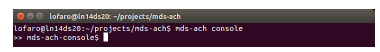Figure 17: Expected window for ($ mds-ach console)

Commands:

This section shows the commands available to the MDS-Console. Note: when in MDS-Console the console will shows the following in the terminal:

Bash/MDS-Ach Console:

>> mds−ach−console$

Function: goto:

The goto command will tell the joint (in joint space) what position (in radians) where to go. The usable joints and abbreviations can be found in Table 2.

Bash/MDS-Ach Console:

>> mds−ach−console$                goto <joint > <value>

This will set the Right Shoulder Pitch (RSP / RightShoulderExt) to a value of -0.123 rad. The expected terminal can be seen in Figure 18.

Bash/MDS-Ach Console (Example):

>> mds−ach−console$              goto RSP −0.123

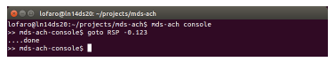Figure 18: Expected window for (>> mds-ach-console$ goto < joint > < value >) using example (>> mds-achconsole$ goto RSP -0.123)

The “get” command gets the joint space position of the < joint > in radians. The usable joints and abbreviations can be found in Table 2. Function: get:

Bash/MDS-Ach Console:

>> mds−ach−console$              get <joint >

This will get the reference and state of the Torso yaw (WST / TorsoPan). The expected terminal can be seen in Figure 19.

Bash/MDS-Ach Console (Example):

>> mds−ach−console$            get WST

Figure 19: Expected window for (>> mds-ach-console$ get < joint >) using example (>> mds-ach-console$ get WST)

Function: get fk:

The “get fk” command gets the work-space position of the left or right end-effector in 6 DOF coordinates (meters and radians) with the origin being the intersection of the robot’s neck and shoulder. The < arm > options are: left and right for the left and right arm respectively.

Bash/MDS-Ach Console:

Bash/MDS-Ach Console (Example):

>> mds−ach−console$           get    fk   l e f t

This will get the 6 DOF work space position of the left end-effector. The expected terminal can be seen in Figure 20.

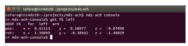Figure 20: Expected window for (>> mds-ach-console$ get fk < arm >) using example (>> mds-ach-console$ get fk left) where (pos) is the position in meters and (rot) is the rotation about x,y,z in radians.

Function: ik:

Bash/MDS-Ach Console:

>> mds−ach−console$                                    ik <arm> <dof> <param 1> . . . <param N>

The “ik” command utilizes the inverse kinematic controller (mds ik module) to solve 1-6 DOF inverse kinematic solutions for the MDS robot’s left or right end-effector. This module uses the Inverse Jacobian Inverse Kinematic solver method. If the desired workspace location is too far away such that the IK controller cannot reach it in 1000 iterations, it will discontinue attempting to find a solution and return without a reply. You may then try another point closer to that of the current end-effector point. < arm > : has the options of “left” and “right.” and denote the left and right end-effector respectively.

< dof > : denotes the number of degrees of freedom you will be controlling using the inverse kinematic controller.

< param 1 > … < param N > : denotes the positions and orientations for the < arm >. The number of parameters must equal that of < dof >. The order must be as follows (Table 5):

Table 5: Inverse Kinematic Parameter Order

Param #	Definition	Abbreviation
1	Position in X	px
2	Position in Y	py
3	Position in Z	pz
4	Rotation in X	θx
5	Rotation in Y	θy
6	Rotation in Z	θz

Bash/MDS-Ach Console (Example):

>> mds−ach−console$           get     fk <arm>

>> mds−ach−console$            ik    l e f t    3 0.3     0.2    0.0

This will find a joint space solution using IK methods for the desired end-effector position to be (0.3 m, 0.2 m, 0.0 m) in (x,y,z). The angle about all axes is in the null space.

The expected output (with running get fk left before and after to show the effect) can be seen in Figure 21.

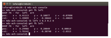Figure 21: Expected window for (>> mds-ach-console$ ik < arm > < dof > < param 1 > … < param N >) using example (>> mds-ach-console$ ik left 3 0.3 0.2 0.0)

E Software Interface

The MDS-Ach system currently works with the C/C++ and Python programming languages. This section describes the required libraries for each of the latter languages.

Python imports:

The following are required imports for the MDSAch system while using python: mds ach, ach, and mds. Other imports are for the given controller implementation.

Python:

# ! / usr / bin / env python import mds ach as mds import ach

C/C++ includes:

The following are required imports for the MDSAch system while using python: mds ach, ach, and mds. Other imports are for the given controller implementation.

C/C++:

#include <mds.h>

#include <ach .h>

Required library:

MakeFile:

−lach

C/C++ MakeFile example with required libraries: The following is an example make file for a C implementation of a controller. Please note it utilizes the required -lach library.

MakeFile:

default :         all CFLAGS := −I ./ include −g −std=gnu99 CC :=       gcc BINARIES := mds−simple−demo LIBS := −lach −l r t −lm all : $(BINARIES) mds−simple−demo:              src /mds−simple−demo. o $(CC) −o $@ $< $( LIBS ) %.o :    %.c $(CC)         $(CFLAGS) −o $@ −c $< clean : rm −f $(BINARIES) src /*. o

F Operating in Joint-Space

This section shows you how to setup the Ach channels for communication with the MDS-Ach system and how to control the robot in joint-space while using the smoothing filter process.

F.1        Control one joint/DOF (Python)

This section shows you how to setup the Ach channels for communication with the MDS-Ach system and how to control one joint of the robot in joint-space while using the smoothing filter process. Specifically we will set the joint-space values as those seen in Table 6. Note that to run this example you will need the libraries for MDS-Ach as seen in Section E.

Table 6: Set the joint space values for the following joint

Name	Alternate Name	Value (rad)
LSP	LeftShoulderExt	-0.123

Open Ach Channels:

Ach channels are how you communicate with MDSAch. You simply write data to the channel and the robot can read the data in newest to oldest order. The section below shows you how to open an Ach channel. Please note that ach.Channel() takes a string as an input. Here we opened two channels:

• s : state channel
• r : reference channel Python:

s = ach . Channel (mds.MDS CHAN STATE NAME) r = ach . Channel (mds.MDS CHAN REF NAME)

Create Required Data Structures:

C-Type data structures are used to pass data between our controllers. Below we create three well defined structures for the state and the reference channels. These structures are defined in mds ach.py and mds.h which is located in your python and include paths.

• state : state channel of type MDS STATE
• ref : reference channel of type MDS REF

Python:

state = mds.MDS STATE() ref = mds.MDS REF()

Get Joint ID:

To command a joint you must get the ID of the joint. The ID numbers are defined in the anatomy.xml configuration file. You can use the joint abbreviations in Table 18 to find the ID number.

Python:

# Get address of LSP jntn = mds. getAddress ( ’LSP ’ , state ) print ’ Address = ’ , jntn

Queue New Motor Position:

You can set a new desired motor angle by setting the reference channel. In this case we are using the filter channel which is the safest one to use due to the velocity and acceleration limiting. Please note that this does NOT send the command to the motor. It queues the values for them to be sent to the motors. They are only sent to the motors after they are “put” on the ach channel.

In the example below we are setting the ‘LSP’ by using the ID number from above to a joint-space angle of -0.123 rad.

Python:

#     Set LSP       reference        to −0.123      using    the # f i l t e r c ontr oll er ref . joint [ jntn ] . ref = −0.123

Set Motor Position (put):

Once all joints are set in the structure you can “put” it on the proper ach channel. Please note that even if you did not set a motor value it will still be put on the channel along with the rest of the data structure. It is best practice to read the latest channel, then modify what you want to change, then put the modified structure on the channel. This will help with not sending the robot to unintended configurations.

Python:

# Command motors to desired # ( post to ach channel ) r . put ( ref )

references

Close Ach Channels on Exit:

Though not required it is good practice to close your unused ach channels upon exit of your controller.

Python:

# Close channels s . close () r . close ()

Running the Code: To run the code do the following from within the mds-ach/examples directory Bash:

$ python mds simple demo python 1 DOF . py

The expected terminal out can be seen in Figure 22.

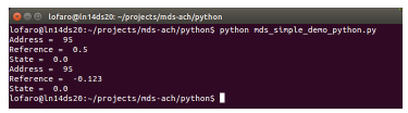Figure 22: Expected window for the python 1-DOF example including additional print statements

You can also monitor the change using the MDSAch Read utility and/or the simulator/real robot.

Full Code:

The full example can be found below as well in the file:

mds-ach/examples/mds_simple_demo_python_1_DOF.py

F.2         Control Two joints/DOF (C/C++)

This section you will set 2 separate DOFs to two different values and see the results. Specifically we will set the joint-space values as those seen in Table 7. Note that to run this example you will need the libraries for MDS-Ach as seen in Section E. We will set the following:

Table 7: Set the joint space values for the following joint

Name	Alternate Name	Value (rad)
LEP	LeftElbowFlex	-0.2
RSP	RightShoulderExt	0.1

Open Ach Channels:

Ach channels are how you communicate with MDSAch. You simply write data to the channel and the robot can read the data in newest to oldest order. The section below shows you how to open an Ach channel. Please note that ach.Channel() takes a string as an input. Here we opened three channels.

• chan state : state channel
• chan ref : reference channel C/C++:

int         r = ach open(&chan ref , MDS CHAN REF FILTER NAME, NULL) ; assert ( ACH OK == r ) ; r = ach open(&chan state , MDS CHAN STATE NAME, NULL) ; assert ( ACH OK == r ) ;

Create Required Data Structures:

C-Type data structures are used to pass data between our controllers. Below we create three well defined structures for the state and the reference channels. These structures are defined in mds ach.py and mds.h which is located in your python and include paths.

• state : state channel of type MDS STATE
• ref : reference channel of type MDS REF C/C++:

mds ref t H ref ; mds state t H state ; memset( &H ref , 0 , sizeof ( Href ) ) ; memset( &H state , 0 , sizeof ( Hstate ) ) ;

Get Up-To-Date Reference:

It is important that you set your initial reference structure with the current values of the reference channel. This is because when you do command the joints you command them all at once, even if you did not change their value. See below for how to get the latest reference values.

C/C++:

int             r = ach get ( &chan ref , &H ref , sizeof ( H ref ) , &fs , NULL, ACH O LAST       ) ; if (ACH OK != r ) { if (debug) { fprintf ( stderr , ”Ref r = %s\n” , ach result to string ( r ) ) ; } } else { assert (            sizeof ( H ref ) == fs ) ; }

Get Joint ID:

For the moment when using C/C++ the joint IDs are hard coded in the mds.h include file. You may use normal humanoid acronyms or NRL legacy acronyms. Queue New Motor Positions:

You can set a new desired motor angle by setting the reference channel. In this case we are using the filter channel which is the safest one to use due to the velocity and acceleration limiting. Please note that this does NOT send the command to the motor. It queues the values for them to be sent to the motors. They are only sent to the motors after they are “put” on the ach channel.

In the example below we are setting the joints as defined in Table 7.

C/C++:

Href . joint [LEP ] . ref = −0.2; Href . joint [RSP ] . ref = 0.1;

Set Motor Position (put):

Once all joints are set in the structure you can “put” it on the proper ach channel. Please note that even if you did not set a motor value it will still be put on the channel along with the rest of the data structure. It is best practice to read the latest channel, then modify what you want to change, then put the modified structure on the channel. This will help with not sending the robot to unintended configurations.

C/C++:

/* Write to the feed −forward channel */ ach put ( &chan ref , &H ref , sizeof ( H ref ) ) ;

Running the example:

To run the example compile then run the resulting executable mds-simple-demo.

Bash:

$      ./mds−simple−demo

The resulting output can be seen using the MDSAch Read utility (Figure 7) and/or the simulator/real robot (Figure 8).

Full Code:

The full example can be found in the file: mds-simple-demo/src/mds-simple-demo.c

G  Built-in IK Controller (C/C++)

The MDS-Ach system has a built-in inverse kinematics

(IK) controller for both the right and left arms. This controller automatically runs when the MDS-Ach system is started. The controller solves for one arm at a time.

The system works by starting to solve the IK equations when you post a new desired position on the IK reference channel. Below is a step by step of how you do this using C/C++.

C/C++ Includes:

The following are required imports for the MDSAch system while using python: mds.h and ach.h. Other imports are for the given controller implementation.

C/C++:

/ /    for   mds

#include <mds.h> / / for ach

#include <ach .h>

Create Open Ach Channel for IK:

Ach channels are how you communicate with MDSAch. You simply write data to the channel and the robot can read the data in newest to oldest order. The section below shows you how to open an Ach channel. Please note that ach open() takes a string as an input. Here we opened one channel. This is a different channel then found in previous sections because it is only for the IK controller.

C/C++:

// open ik         chan int         r = ach open(&chan ik , MDS CHAN IK NAME, NULL) ; assert ( ACH OK == r ) ;

Make IK Structure:

Similar to controlling the robot in joint-space you need to set a reference structure to the desired workspace position. For this you need to initialize the structure. See below for the initialization of the work-space structure.

C/C++:

/ / Make new IK structure mds ik t H ik ; memset( &H ik , 0 , sizeof ( H ik ) ) ;

Setting the DOF controlled:

When using the built-in IK controller you need to set the number of DOF that you are controlling. With this controller you are required to set the DOF in the following order: p_x,p_y,p_z,θ_x,θ_y,θ_z where p_n is the position on axis n and θ_n is the rotation about axis n. For example if you DOF is set to 4 you are controlling p_x,p_y,p_z, and θ_x. If you are controlling 2 you will control p_x and p_y. In the example below we are controlling 3, i.e. p_x,p_y, and p_z. This order can also be seen in Table 5.

C/C++:

/ / Set the amount of DOF you want to control dof = 3

We set these to the values in Table 3.

θ_x,θ_y, and θ_z are in the Null Space because we do

not care where they are as long as the first three parameters are met. We can set these values to what ever we want and they will be ignored. In this case we set them to zero.

C/C++:

/* Set      values     for     work−space     in [x , y , z , rx , ry , rz ] order */ double eff [6] = {0.3 , 0.2 , 0.0 , 0.0 , 0.0 ,

0.0};

Choosing Arm for IK:

Here we pick the arm for the IK. Our options are set as enums in the mds.h include. All options for right and left arms can be found in Table 8.

Table 8: Definitions for left and right arms using mds ach.py in Python

Arm	C/C++ Definition
Left	LEFT
Right	RIGHT

Here we set the arm to the left arm.

C/C++:

/ / set arm int arm = LEFT;

Set IK Structure:

Just as in the joint-space method, we need to the values in our structure before we send it to the robot. Here we set all of the parameters from above to the structure ikc that we created.

C/C++:

/ / Put setting into ik structure Hik .move = arm; Hik .arm[arm ] . ik method = dof ; Hik .arm[arm ] . t x = eff [ 0 ] ; Hik .arm[arm ] . t y = eff [ 1 ] ; Hik .arm[arm ] . t z = eff [ 2 ] ; Hik .arm[arm ] . r x = eff [ 3 ] ; Hik .arm[arm ] . r y = eff [ 4 ] ; Hik .arm[arm ] . r z = eff [ 5 ] ;

Command the Robot:

Just as with the joint-space controller you need to “put” the data on the ACH channel. Unlike the jointspace controller it will not move as soon as you send it. The controller will first have to solve the IK. Upon finding the solution the controller will send it to the robot. If a solution is found it will take anywhere between 0.1 and 5.0 seconds. If there is no solution found the robot will not move. Note: the robot limits its self to 1000 search iterations for an IK solution.

C/C++:

/ / put on to ACH channel ach put ( &chan ik , &H ik ,

sizeof ( H ik ) ) ;

Running the Code:

To run the code do the following within the mdssimple-demo-ik folder.

Bash:

$ make clean

$ make

$      ./mds−simple−demo−ik

To check that the IK worked you can run the FK in the MDS-Ach console and/or run the simulator. The before and after of the MDS-Ach console is found in Figure 23 and Figure 24 respectively.

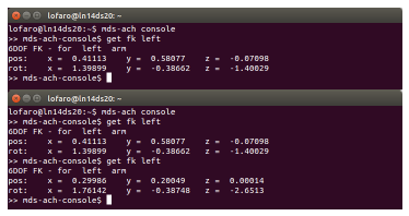Figure 23: Expected MDS-Ach Console window for (>> mds-ach-console$ get fk left). (TOP) Before running. (BOTTOM) After running.

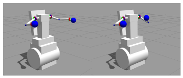Figure 24: Expected simulator window for ($ ./mds-simple-demo-ik) and/or ($ python mds ik solver example.py). (LEFT) Before running. (RIGHT) After running.

Full Code:

The full example can be found in the file: mds-simple-demo/src/mds-simple-demo-ik.c

H Inverse Kinematics API

This section will show you an example of how to get and set the forward and inverse kinematics via the mds ik API. The goal of this tutorial is to solve for the joint-space values given the desired work-space values as found in Table 3. This API is written for use with Python but also has hooks for C/C++.

Required Imports:

Below are the required imports for using the forward/inverse kinematics portion of the mds API. These will be located in the python 2.7 path.

Python:

import mds ach as mds import ach import mds ik as ik import mds ik include as ike from mds ach import *

Open Ach Channels:

You will need the state and the reference (filtered) channels to solve and set the IK using the API. The state is used to get the current location of the robot. The reference is used to set the joint-space values once they are found.

Python:

# Open Ach Channels

r = ach . Channel (mds.MDS CHAN REF FILTER NAME) s = ach . Channel (mds.MDS CHAN STATE NAME)

Make Structures:

Make the structures for the state and the reference channels. This will hold your latest state data and the latest set reference to the reference filter channel.

Python:

# Make Structs state = mds.MDS STATE() ref = mds.MDS REF()

Get Latest Data:

Get the latest data from the state and reference channels.

Python:

# Get     the	l a t e s t     on   the     channels
[ status ,	framesize ] = s . get ( state , wait=False , last=True )
[ status ,	framesize ] = r . get ( ref , wait=False , last=True )

Set Desired Work-Space Position:

Set the desired work-space position as found in Table 3. We set all 6 DOF here however only the first three are required due to our desired work-space position. Later sections removes the extra DOFs.

Python:

# Desired position eff end = np. array ([0.3 ,0.2 ,0.0 ,0.0 ,0.0 ,0.0])

Set Desired Arm:

The ik.getIK() function takes a string to define the left or right arm. Thus we set our “arm” as a string. The options for the latter can be found in Table 9.

Table 9: Definitions for left and right arms using mds ik.py in Python

Arm	MDS IK (Python) Definition
Left	’left’
Right	’right’

Python:

# Define Arm arm = ’ l e f t ’

Get Current Joint-Space Pose:

Next we have to get the current joint-space pose of the robot and putting it into a 6 DOF array. This is done by looking for the index of each joint and then putting them in an array. The array must be in the order defined in Table 10.

Python:

# Get current joint space pose of arm jntn = mds. getAddress ( ’LSP ’ , state ) j0 = state . joint [ jntn ] . ref jntn = mds. getAddress ( ’LSR ’ , state ) j1 = state . joint [ jntn ] . ref jntn = mds. getAddress ( ’LSY ’ , state ) j2 = state . joint [ jntn ] . ref jntn = mds. getAddress ( ’LEP ’ , state ) j3 = state . joint [ jntn ] . ref jntn = mds. getAddress ( ’LWY’ , state ) j4 = state . joint [ jntn ] . ref jntn = mds. getAddress ( ’LWR’ , state ) j5 = state . joint [ jntn ] . ref eff joint space current =[j0 , j1 , j2 , j3 , j4 , j5 ]

Table 10: Arm joint-space pose order.

Array	Joint	Short Name	Short Name
Index	Definition	(left)	(right)
0	Shoulder Pitch	LSP	RSP
1	Shoulder Roll	LSR	RSR
2	Shoulder Yaw	LSY	RSY
3	Elbow Pitch	LEP	REP
4	Wrist Yaw	LWY	RWY
5	Wrist Roll	LWR	RWR

Set DOF and Order of Desired Work-Space Position:

We now set the DOF of the desired work-space (acceptable numbers are 1-6) and the order in which we input them. Using the MDS IK API we can input the desired work-space coordinates in any order we desire. The order is defined by an array of string that we call

‘order’. The valid inputs for this array can be found in Table 11.

Table 11: Valid Inputs for “order” Array

Definition	Input to Array (String)
Position in x (px) (meters)	’p x’
Position in y (py) (meters)	’p y’
Position in z (pz) (meters)	’p z’
Rotation about x (θx) (radians)	’t x’
Rotation about y (θy) (radians)	’t y’
Rotation about z (θz) (radians)	’t z’

Here we have 3 DOF with an order of position in x, y, then z. Note: This order MUST match that of the order in your desired work-space position array in Section H.

Python:

# set the dof and the order dof = 3 order = [ ’ p x ’ , ’ p y ’ , ’ p z ’ ]

( dof = 3)

Set Error:

Here we set the error for the IK solver. The error is a 3D array with the atrobutes found in Table 12.

Table 12: Error Array Index Definitions

Index	Definition
0	Max change in angular position (θ) per iteration (rad)
1	Max change in linear position (xyz) per iteration (m)
2	Max linear Error (m2 +rad2)

The max change in angular position is the maximum distance in radians that the solver will move per iteration. The max change in translational position is the maximum distance translated in x,y,z per iteration in meters. The max linear error (e_max) is the linear distance in N DOF that disregards units. The error in the end-effectors actual position vs its desired position (e_{ef f} ) can be found via the equation below.

where d_des is the desired pose and d_act is the actual pose. The system will say the IK has been solved if

eef f ^≤ emax.

To set the desired errors make the 3D array as seen below. If no error is input the default values of [0.01,0.01,0.01] will be used.

Python:

# set the allowable error err = np. array ([0.01 ,0.01 ,

0.01])

Set Max Solving Iterations:

Due to the nature of the IK method utilized the system can fall into local minimum or a hysteresis. This will cause the system to attempt to solve indefinitely. To avoid this use add a maximum number of iterations to try when solving the IK. This number is set below.

If not set it will use the default value of 1000.

Python:

# Set solving step number max stepNum = 1000

Limit input to desired DOF:

Here you limit the size of the desired end-effector position vector to the ‘dof’ that we defined in Section H.

Python:

# Deisred position for only eff end = eff end [ : dof ]

the

dof we want

Solving the IK:

Now we can solve the IK via the use of ik.getIK() in the mds ik python module.

Python:

# Solve IK jnt return = ik . getIK ( eff joint space current , eff end ,     order ,      arm , err , stepNum)

The output of this is a 2D array where index 1 returns a -1 if there is no IK solved. Index 0 is the array of the end-effectors joint-space values for the given desired work-space position. The order of the joint-space values are the same as what is found in Table 10.

Python:

#              returns     in             the                following  order #     Joint                space       return = # [LSP , LSR , LRY, LEP , LWY, LWR] eff joint space current = jnt return [0]

Putting the IK solution on the robot:

To put the IK solution on the robot we map the received joint space values on the reference (ref) structure of the robot’s MDS-Ach system. Again the order of the joint-space values are the same as what is found in Table 10. In this case we are setting the left arm.

Python:

# Set to joint space jntn = mds. getAddress ( ’LSP ’ , state ) ref . joint [ jntn ] . ref=eff joint space current [0] jnt n= mds. getAddress ( ’LSR ’ , state ) ref . joint [ jntn ] . ref=eff joint space current [1] jntn = mds. getAddress ( ’LSY ’ , state ) ref . joint [ jntn ] . ref=eff joint space current [2] jnt n= mds. getAddress ( ’LEP ’ , state ) ref . joint [ jntn ] . ref=eff joint space current [3] jntn = mds. getAddress ( ’LWY’ , state ) ref . joint [ jntn ] . ref=eff joint space current [4] jntn = mds. getAddress ( ’LWR’ , state ) ref . joint [ jntn ] . ref=eff joint space current [5]

Commanding the robot:

Just as in previous sections, we have to “put” the resulting structure on the reference (filtered) channel before the robot will move. Please note that we are using the filtered channel the the robot will not “jerk” during the joint-space step input operation.

Python:

# Send    to    the r . put ( ref )

robot

Getting the Forward Kinematics from joint-space pose:

We can get the work-space position of the arm via the forward kinematics (FK) by utilizing the joint-space pose the the ik.getFkArm() function of the mds ik module.

Python:

#      get FK of      arm A = ik . getFkArm( eff joint space current ,arm) eff end ret=ik . getPosCurrentFromOrder (A, order )

ik.getFkArm() will return a 4×4 matrix which includes the rotation and translations components. The ik.getPosCurrentFromOrder() returns the work-space position and orientation in the same order as requested by “order”. This will return a 1xN array where N is equal to the length of your “order”. You can find the error by doing the following.

Python:

# find d i f f e r e n t in desired vs actuial eff end dif = eff end − eff end ret

pos

Running the code:

To run the code enter the “examples” directory of the mds-ach project and run the following command: Bash:

$ python            mds ik solver example . py

The resulting console output should look like Figure 25.

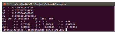Figure      25:        Expected      window     for     ($      python mds ik solver example.py)

1.  M. Quigley, K. Conley, B. P. Gerkey, J. Faust, T. Foote, J. Leibs, R. Wheeler, and A. Y. Ng, “Ros: an open-source robot operating system,” in ICRA Workshop on Open Source Software, 2009.
2.  C. Breazeal, M. Siegel, M. Berlin, J. Gray, R. A. Grupen, P. Deegan, J. Weber, K. Narendran, and J. McBean, “Mobile, dexterous, social robots for mobile manipulation and human-robot interaction,” in International Conference on Computer Graphics and Interactive Techniques, SIGGRAPH 2008, Los Angeles, California, August 11-15, 2008, New Tech Demos Proceedings. ACM, 2008, p. 27. [Online]. Available: http://doi.acm.org/10.1145/1401615.1401642
3.  Y. Maruyama, S. Kato, and T. Azumi, “Exploring the performance of ros2,” in Proceedings of the 13th International Conference on Embedded Software, ser. EMSOFT ’16. New York, NY, USA: ACM, 2016, pp. 5:1–5:10. [Online]. Available: http://doi.acm.org/10.1145/2968478.2968502
4.  D. Calisi, A. Censi, L. Iocchi, and D. Nardi, “OpenRDK: a framework for rapid and concurrent software prototyping,” in Proceedings of Int. Workshop on System and Concurrent Engineering for Space Applications (SECESA), Nov. 2008.
5.  T. H. J. Collett and B. A. Macdonald, “Player 2.0: Toward a practical robot programming framework,” in in Proc. of the Australasian Conference on Robotics and Automation (ACRA, 2005.
6.  G. Metta, P. Fitzpatrick, and L. Natale, “Yarp: Yet another robot platform,” International Journal of Advanced Robotics Systems, special issue on Software Development and Integration in Robotics, vol. 3, no. 1, 2006.
7.  C. Ct, Y. Brosseau, D. Ltourneau, C. Raevsky, and F. Michaud, “Robotic software integration using marie,” International Journal of Advanced Robotic Systems, vol. 3, no. 1, pp. 055–060, March 2006. [Online]. Available: http://www.ars-journal. com/International-Journal-of-Advanced-Robotic-Systems/ Volume-3/055-060.pdf
8.  N. Ando, T. Suehiro, K. Kitagaki, T. Kotoku, and W.-K. Yoon, “RT-Component Object Model in RT-Middleware Distributed Component Middleware for RT (Robot Technology),” pp. 457–462, Jun. 2005.
9.  A. Makarenko and A. Brooks, “Orca: Components for robotics,” in In 2006 IEEE/RSJ International Conference on Intelligent Robots and Systems (IROS 2006), 2006.
10.  M. Henning, “A new approach to object-oriented middleware,” IEEE Internet Computing, vol. 8, no. 1, pp. 66–75, Jan 2004.
11.  S. Rowe and C. R. Wagner, “An introduction to the joint architecture for unmanned systems (jaus),” Ann Arbor, vol. 1001, p. 48108.
12.  N. Dantam, D. Lofaro, A. Hereid, P. Oh, A. Ames, and M. Stilman, “The ach library: A new framework for real-time communication,” Robotics Automation Magazine, IEEE, vol. 22, no. 1, pp. 76–85, March 2015.
13.  D. M. Lofaro, C. Ward, M. Bugajska, and D. Sofge, “Extending the life of legacy robots: Mds-ach, a real-time, process based, networked, secure middleware based on the x-ach methodology,” in 15th InternationalWorkshop on Advanced Motion Control (IEEE-AMC2018), March 2018.
14.  A. Perez, M. Orsag, and D. Lofaro, “Design, implementation, and control of the underwater legged robot aquashoko for low-signature underwater exploration,” in 2018 15th IEEE International Conference on Ubiquitous Robots (UR), 2018.
15.  J. Brown and B. Martin, “How fast is fast enough? Choosing between Xenomai and Linux for real-time applications,” in Twelfth Real-Time Linux Workshop on October 25 to 27, in Nairobi, Kenya, 2010.
16.  N. Koenig and A. Howard, “Design and use paradigms for gazebo, an open-source multi-robot simulator,” in IEEE/RSJ International Conference on Intelligent Robots and Systems, Sendai, Japan, Sep 2004, pp. 2149–2154.
17.  R. Smith, “Open dynamics engine,” 2008. [Online]. Available: http://www.ode.org/
18.  S. R. Buss, “Introduction to inverse kinematics with jacobian transpose, pseudoinverse and damped least squares methods.”
19.  D. Lofaro, R. Ellenberg, P. Oh, and J. Oh, “Humanoid throwing: Design of collision-free trajectories with sparse reachable maps,” in Intelligent Robots and Systems (IROS), 2012 IEEE/RSJ International Conference on, Oct 2012, pp. 1519–1524.
20. D. M. Lofaro, “Secure robotics,” in 2016 13th International Conference on Ubiquitous Robots and Ambient Intelligence (URAI), Aug 2016, pp. 311–313.
21.  D. Lofaro, “Mds-ach,” in https://github.com/thedancomplex/mdsach, 2015.

(Click Here)

(Click Here)