1.Introduction

Reliability significantly influences the quality of product. Thus, many manufacturers make great effort to enhance the product reliability that largely determines the product competitiveness. Such importance has brought practitioners’ attention to reliability evaluation. In life data analysis, we have to collect the failure time of a product under normal design conditions to quantify life characteristics of the product. However, such failure data for lifetime are very difficult to obtain in many situations, especially for the product with high reliability. Nowadays, lifetimes of many products are too long and the life testing period between design and release is limited; so, the tests under normal design conditions are too lengthy to get any failures. To overcome this problem, accelerate life testing (ALT) has been developed.

Since ALT can shorten the lifetime of a product, we often adopt it in order to obtain the failure information quickly within a limited time frame. In an ALT experiment, the test units are generally subjected to the stress levels that are higher than normal design level. The commonly used stress factors for failure acceleration include temperature, vibration, voltage, and pressure. Both the use of specific accelerated stress factors and the range of stress levels for a particular material or product are often suggested by engineering practice. Then, the failure data obtained at accelerated conditions have to be extrapolated through a proper model so that the characteristics of life distribution at normal design conditions can be estimated. A number of different types of stress loading schemes (such as constant, cyclic, step, progressive, and random stress loading) are available in practice when performing an ALT. By the relation between the stress levels and testing time, these stress loading schemes can be classified into two categories: time-independent and time-dependent stress loadings. When the stress loading is time-independent such as constant stress loading, the stress level applied to each of the test units stays the same during the entire testing period. One of the demerits of using constant stress loading in ALT is that it could still take too long to run for the test experiment to observe sufficient failures when the inappropriate testing stress levels are applied. To address this problem, a time-dependent stress loading scheme is preferred to assure quick failures. When a time-dependent stress loading, such as step-stress, is adopted, test units are subjected to a stress level that is changing over testing time. In this paper, we consider step-stress ALT where all test units are subjected to the stress levels increasing by steps.

This paper is an extension of our previous work [1] originally presented in The Third IEEE International Conference on World Computing and Big Data Analysis. In literature, almost all the previous works done by others for Cox’s proportional hazards (PH) based ALT models are very limited on simple step-stress assuming the baseline hazard function is simple linear. However, [2] have indicated that the optimal multiple step-stress ALT may further improve the quality of the reliability pre  diction for a parametric model. Therefore, this paper broadens the results of [1] where has only addressed the optimal ALT plans for PH models with a linear baseline function and moves on to discussing multiple step-stress optimal designs for ALT when adopting a PH model with either a simple linear or a quadratic baseline hazard function. In this paper, both optimal stress levels and optimal stress-changing times for three-step-stress ALT designs are derived under three different optimality criteria.

2. Literature Review and Preliminaries

2.1.  Optimal designs for step-stress ALTs with a non-PH model

Miller and Nelson [3] first discussed Q-optimal designs for simple step-stress ALT tests with complete failure data assumed to be exponentially distributed. Their optimal designs were attained by minimizing the asymptotic variance (AVAR) of the maximum likelihood estimator (MLE) of the mean lifetime at the normal design stress level. Then, their work was extended to censored data by [4] who obtained the optimal simple step-stress ALT designs incorporating time-censoring. For some products or material, their failure times often follows a Weibull distribution. Assuming a Weibull distribution with a constant scale parameter, both [5] and [6] constructed optimal simple step-stress ALT designs for time-censoring. Bai and Kim in [5] obtained the optimal low stress level and optimal stress-changing time in order to minimize the AVAR of the MLE of a specific quantile of the product’s lifetime distribution at the normal design stress level whereas [6] obtained their optimal stress-changing time in order to minimize the AVAR of the MLE for reliability prediction instead. In addition, Hunt and Xu in [7] further investigated optimal simple step-stress ALT plans for a Weibull distribution; however, they assumed both the shape and scale parameters were functions of the stress levels. Their resulting optimal designs chosen the stress-changing time in order to minimize AVAR of the MLE of reliability prediction at the normal design stress level and at a pre-specified time. They also reviewed the research work on optimal designs for step-stress ALT. Please see the references therein. We note that all these work previously done had provided the design construction methods only for simple step-stress ALT plans.

Moreover, Ma and Meeker in [8] extended the research by [5] to provide a general method for multiple step-stress ALTs assuming a log-location-scale family of distributions. They discussed an approach to calculate the large-sample approximate variance of the MLE for a percentile of the failure time distribution at normal design conditions when the failure data were observed from a step-stress ALT. By adopting a cumulative exposure model, their approach allowed for both multiple step-stress loading and censoring. Their results also showed that depending on the values of the model parameters and certain percentile of interest, one of the three test plans proposed could be the most preferable in terms of optimum variance. For a Weibull lifetime distribution, however, with possible inaccuracy in the assumed log-linear life-stress [2] investigated the optimal stress-changing time for simple step-stress ALT plans in order that the asymptotic mean squared error of the underlying reliability estimator could be minimized, and the robust choices of three-step-stress plans were also discussed with the awareness of possible imprecision in the assumed life-stress relationship by minimizing the asymptotic squared bias.

2.2.  Optimal designs for constant stress or simple step-stress ALTs with a PH model

Jiao in [9] first investigated the optimal design problem for a PH model when a constant-stress ALT experiment being planned, and then developed the optimal designs for reliability prediction by optimally choosing both stress levels and proportion of units allocated to each stress level in order to attain the most accurate reliability estimate at normal design conditions. Moreover, when a step-stress ALT experiment was planned, [9] discussed the simple step-stress ALT plan for reliability prediction and obtained the optimal stress level by minimizing the variance of the MLE of hazard rate at the normal design stress level and over a pre-specified time period. In addition, [9] also provided an algorithm for solving the constrained nonlinear optimization problems.

On the other hand, Elsayed and Zhang in [10] revealed an optimal simple step-stress ALT plan so as to obtain the most accurate reliability function estimates at normal design conditions. They also formulated a nonlinear programming problem to minimize the asymptotic variance of the hazard rate estimator over a prespecified the period at the normal design stress level. More recently, Hu, Plante, and Tang in [11] briefly discussed the optimal low and high stress levels in a simple step-stress ALT in order to minimize the mean squared error of the estimated upper confidence bound for the cumulative failure probability of a product at normal design conditions, with a given stress-changing time. In sum, all these existing works provided the methods of optimal design construction only for simple step-stress ALT plans. Therefore, we expand the previous work of others and investigate the optimal designs of multiple step-stress ALT for PH models in this paper.

2.3.  Optimal designs for general proportional hazards models

There is broader literature of optimal designs available for general proportional hazards models, which are not necessary with consideration of step-stress ALT plans. To name a few, Becker, McDonald, and Khoo in [12] constructed D-optimal designs for proportional hazards models with one or two parameters when its baseline hazard function was specified. They developed the method of minimum variance design construction when various censoring schemes were adopted. Dette and Sahm  in [13] provided a standardized maximum variance design criterion which could be applied to obtain the optimal designs whereas McGree and Eccleston in [14] created compound criteria so that optimal designs could be derived for multi-objective scenarios. L´opez-Fidalgo, Rivas-L´opez, and Del Campo in [15] also proposed an algorithm to find optimal designs for typical Cox regression models incorporating censoring. More recently, Konstantinou, Biedermann, and Kimber investigated the general maximin D-optimal designs for a class of models and discussed the application of their design construction method to the proportional hazards models in [16].

2.4.  Our model and some preliminaries

One of the most commonly used means for predicting the lifetime of a product is Cox’s PH model since it provides sufficient flexibility for identifying the effects of covariates on the failure rate. In this paper, a PH model with hazard ratio being independent of time is considered. Therefore, the hazard rate of a product can be expressed

where is a baseline hazard function,  is a column vector of unknown parameters, and  is a column vector of the covariates (applied or transformed stresses) for an ALT experiment, and that are independent of the baseline hazard. Presumably, the stresses are having multiplicatively effects on the hazard rate in this model.

We conduct ALT with step-stress loading where all the test units begin at a prespecified stress level. After a time fraction, the stress level is changed to a higher stress level. The stress level can be raised more than once before the test completes. A simple step-stress ALT, also called a two-step-stress ALT, only uses two stress levels during an ALT experiment. In contrast, in multiple step-stress ALT, more than two stress levels are needed and the stress level is raised at least twice before the test ends. In this paper, we discuss multiple step-stress ALT experiments. We denote by  the normal design stress level. For a three-step-stress, we signify the low, middle and high stress levels by , , and , the stress-changing times by  and , and censoring time by .

In this paper, we assume  to be in either a linear or a quadratic form. For either case, we investigate the optimal three-step-stress ALT design construction under D-optimality, A-optimality, and Q-optimality, respectively. We obtain D-optimal designs in order to minimize the determinant of covariance matrix of the estimators for the model parameters (or equivalently maximize the determinant of Fisher’s information matrix), A-optimal designs in order to minimize the trace of covariance matrix of the estimators for the model parameters, and Q-optimal design to minimize the asymptotic variance of the estimator for a specific quantity of interest. The major quantity of interest in this paper is the average hazard rate over a particular period of time under normal design conditions.

For the case of  being simple linear, the main part of the optimal design construction was presented in [1]. Therefore, we will only restate the necessary notations being continuously used here and also summarize the previous results for comparison purpose in this paper. For the case of  being a quadratic function, we will present the discussion and derivation in full. Furthermore, because there was no simulation study done previously for either case, we will demonstrate simulation and comparison studies for both cases in the present paper.

The rest of this paper is organized as follows: in Section 3, the optimal three-step-stress ALT design results have been summarized for the case when the baseline hazard function  in (1) is assumed to be a simple linear function. In Section 4, the optimal three-step-stress ALT design have been derived for the case when  is considered to be a quadratic function. The method of the optimal design construction involves the minimization for a nonlinear objective function with nonlinear constraints, and some practical examples are used to illustrate the proposed method for the construction of constrained optimal designs in Sections 3 and 4. We have also evaluated the performance of the resulting designs obtained in both Sections 3 and 4 through simulations and comparisons in Section 5. Some concluding remarks are presented in Section 6.

3. Optimal designs when  being a simple linear function

Xu and Huang in [1] first focused on determining the optimal three-step-stress ALT designs for a PH model with time-censoring in the case when the baseline hazard function is considered being a simple linear function. They have provided detailed derivation for the information matrix and the optimal choices of both the middle stress level and stress-changing times for all cases considered there. For comparison reasons, we keep the same notations which are presented in Subsection 3.1, and their main results are summarized in this section.

3.1.  Notation

Although the method of development for multiple step-stress ALT designs can be provided in general, we formulate our design construction using three-step-stress ALT experiments for its simplicity. A three-step-stress ALT experiment with time-censoring involves a predefined censoring time , and three test stress levels   , and which satisfies  . Assuming there are  test units available for the ALT experiment, they are all first placed at low stress level  for a time interval   . Afterwards, the test units survived by time  are subjected to a middle stress level  for the next time interval    Next, the remaining units by time   are subjected to the highest stress level  for the last time interval    . Then, the test ends at censoring time  We consider Model (1), under a stress level  where  being independent of .

We make use of the notations     , and  to represent the cumulative distribution function (cdf), the probability density function (pdf), the cumulative hazard function, and the reliability function of failure time , respectively, at a given stress level . We also employ the cumulative exposure model (CEM), please see [17] for details, to address the changes of  in lifetime  due to the stress step-ups in a step-stress ALT experiment. We denote the cdf under  by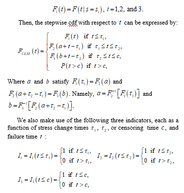

where . Taking a three-step-stress design  with three stress levels being    and , the log-likelihood function of an observed lifetime  can be written as: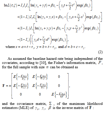

The elements of the Fisher’s information matrix for    are the negative expectations of the corresponding second partial derivatives. We denote the non-zero elements of Fisher’s information by            and   . In [1], Xu and Huang have derived the expressions of these elements as follows:

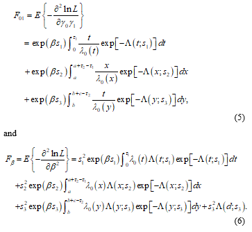
We note that the derivation of these elements in this subsection and the expressions of the loss functions in next subsection have been omitted, please see [1] for details.

3.2.  Loss functions and design constraints

In this paper, we consider the following three different design criteria: D-optimality, A-optimality, and Q-optimality. In [1], Xu and Huang has derived the corresponding three loss functions as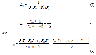

respectively.

In ALT practice, there are often some requirement needed on the minimum number of failures at each stress level. Similarly to [10] for designing optimal simple step-stress ALTs, we take certain practical constraints into consideration in our optimal design construction process for multiple step-stress ALTs. In this paper, we consider three design constraints as below:

The minimum expected number of failures (MNF) at stress level is required as :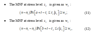where  is the number of failures under each stress level , 

With these constraints, the optimal decision variables ( , ,  ) can be determined by minimizing each of the above-mentioned loss functions. Specifically, we choose the optimal designs in order to minimize (7), (8), or (9) with respect to ( , , ) subject to all three constraints (10), (11), and (12). We denote the optimal designs corresponding to the three optimality criteria by ,  ,  and  , which can be expressed as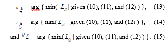

3.3.  Optimal designs when the middle stress being fixed

In [10], Elsayed and Zhang discussed an example of conducting a two-step-stress ALT experiment for metal oxide semiconductor capacitors and estimating the hazard rate over 10 years at design temperature  The total number of test units was n = 200 and the test was censored by c = 300 hours. In order to avoid any unanticipated change in failure mechanisms during the ALT experiment, the maximum testing temperature was determined to be  by the engineering experimenters. The initial values of the model parameters was taken as   ,    and  . The Q-optimal low accelerated stress level was found to be  .

In this subsection, we use this example to compare the optimal two-step-stress ALT designs obtained in [10] with our proposed three-step-stress ALT designs. Previously, the optimal two-step-stress ALT designs are having   and . For our three-step-stress ALT plans, we keep the number of test units, censoring time, and the lowest and highest stress levels all the same. Namely,  n = 200,  c = 300 ,   and  . The initial values for the model parameters are kept the same as well. Conveniently, the experimenters often take  as the average of  and . Therefore, we discuss two scenarios for the choice of  : (a)  being    which is the average of   and  ; and (b) being optimally chosen, together with stress changing times, in order to minimize a specified loss function. We note that when temperature is taken as a stress factor appeared in a PH model for ALT, absolute temperature is often used as its measurement unit for model fitting.

Table 1. Constraint cases for two-step-stress ALT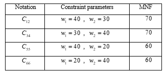

Table 2. Constraint cases for three-step-stress ALT

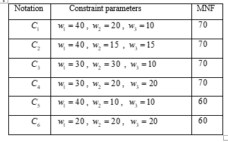In Scenario (a), the optimal stress changing times,  and , can be chosen in order to minimize       , or    under some specific constraints. We take several practical constraint cases with given ,  and , and these cases accompanied by their notations are recorded in Table 1 for two-step-stress ALT designs, and in Table 2 for three-step-stress ALT designs.

We denote the D-, A- and Q-optimal designs obtained for two-step-stress ALT under a given constraint case  by      and , where  k = 12, 34, 55, 66, and the D-, A- and Q-optimal designs obtained for three-step-stress ALT under a given constraint  by    and , where  k = 1, …, 6,  and  i = 1, 2  with  i  referring to the different scenario of   (i = 1 for Scenario (a), and i = 2 for Scenario (b)). Moreover, we define the asymptotic D-, A-, Q-efficiencies of    relative to    as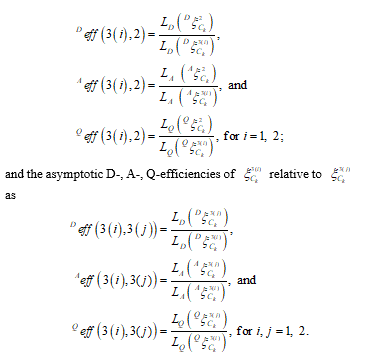

The optimal stress-changing time(s), for both two-step-stress plans and the three-step-stress ALT plans with    being fixed at   are obtained by minimizing       , or  ,  respectively for all the constraint cases considered. We note that the resulting optimal stress-changing times are all the same for these three different optimal criteria although their corresponding relative efficiencies are not the same. The optimal stress-changing times and relative efficiencies for all six constraint cases (as listed in Table 2) are presented in Tables 3 and 4. The overall average efficiency gain after unitizing an optimal three-step-stress plan is 5.44%  when   being fixed at  .

4. Optimal designs when baseline hazard is a quadratic function

4.1.  Preliminary

We have considered the PH based ALT with the case where the baseline hazard function is a simple linear function in Section 3. In many practical situations, this simple model can be under-fitted. Therefore, in this section, we focus on the PH model when the baseline hazard function is in a quadratic form. Namely, we adopt Model (m1) where the baseline hazard function is rather being

Table 3. D-, A-, Q-optimal stress-changing times, when   =

3-step-stress ALT			2-step-stress ALT
optimal designs			optimal designs
	178.2	223.6		183
	178.0	209.2		183
	162.9	219.4		156
	162.1	194.8		156
	198.0	227.5		201
	162.1	194.8		156

Table 4. D-, A-, Q- relative efficiencies, when   =

	1.06	1.04	1.10	1.06	1.04	1.06
	1.06	1.03	1.09	1.06	1.04	1.06
	1.04	1.03	1.08	1.05	1.03	1.05

Consequently, the cdf, pdf, the cumulative hazard function, and the reliability function of failure time t, at a given stress level s, become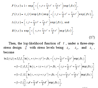

where x, y, and d are defined as in (2). Its first partial derivatives with respect to the model parameters        and    are the same as in (3) but with    being defined as in (16) instead, and the one with respect to    is

Table 5. D-optimal designs and relative efficiencies

3-step-stress ALT, = 155			D-relative efficiency
Optimal design
	152.65	247.44	1.13	1.07
	148.33	226.85	1.09	1.05
	152.93	247.44	1.19	1.09
	143.25	211.74	1.12	1.06
	179.40	245.78	1.08	1.04
	161.43	211.03	1.11	1.05

Table 6. A-optimal designs and relative efficiencies 3-step-stress ALT, = 155 A-relative efficiency Optimal design 155.20 247.47 1.13 1.07 147.99 226.84 1.09 1.06 155.13 247.47 1.19 1.09 142.41 211.73 1.11 1.05 155.18 247.47 1.09 1.05 142.39 211.73 1.11 1.05 Table 7. Q-optimal designs and relative efficiencies 3-step-stress ALT,   = 155 D-relative efficiency Optimal design 156.19 247.47 1.09 1.05 149.81 226.86 1.07 1.04 156.71 247.47 1.14 1.06 144.20 211.75 1.09 1.04 156.45 247.47 1.06 1.03 143.98 211.75 1.09 1.04

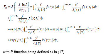
Its second partial derivatives            and    can be expressed as the same as in Xu and Huang (2018) but with their    and    function being defined as in (16) and (17), and their corresponding elements of the Fisher’s information matrix for a single failure time t (the expected value of negative second derivatives) are as the same as in (3), (4), (5), and (6). The remaining second derivatives are

and their corresponding elements of the Fisher’s information matrix for a single t can be derived as below: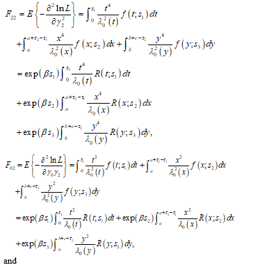

As indicated in Section 3.1, the correlations between the stress coefficient  and baseline parameters  and  are equal to zero. Consequently, the covariance matrix  of the MLEs of  can be expressed as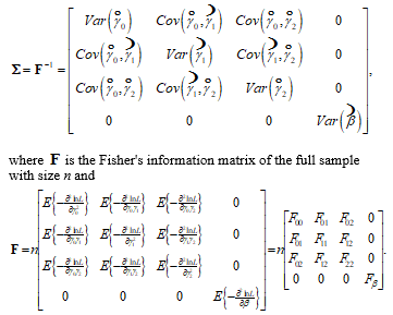

4.2.  Loss functions and design constraints

Now the loss functions under D-, A-, and Q-optimality become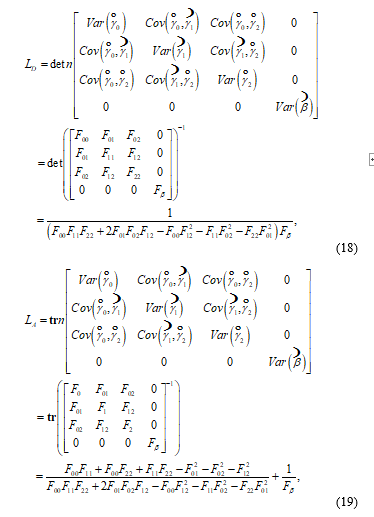

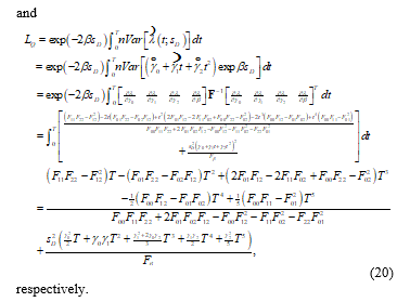
The optimal decision variables (  ,   ,   ) are chosen by minimizing the loss function (18), (19), or (20) with some design constraints. We also keep the three constrains (10), (11), and (12)  as the same as those in Section 3. The corresponding designs ,  and  can also be described as (13), (14), and (15).

4.3.  Optimal three-step-stress designs

In this subsection, we revisit the example presented in Section 3, and discuss the optimal ALT designs when the fitting model is a PH model with a quadratic baseline hazard function. Suppose from previous experience, the initial values for the model parameters are  , , , . All other values of the design parameters in the example remain the same. Thus, the accelerated stress levels remain as ,  Here we also consider the six constraint cases as used in Section 3.

When is conveniently chosen as    the resulting two-step-stress and three-step-stress optimal designs under D-, A, and Q-optimality criteria appeared to be the same again. Nonetheless, the relative efficiencies are not always better than their corresponding peers, the optimal two-step-stress designs. These designs and their relative efficiencies under D-, A-, and Q-optimalities are displayed in Tables 8 and 9, respectively.

Table 8. D-, A-, Q-optimal stress-changing times, when  =

3-step-stress ALT			2-step-stress ALT
optimal designs			optimal designs
	178.2	223.6		183
	178.0	209.2		183
	162.9	219.4		156
	162.1	194.8		156
	198.0	227.5		201
	162.1	194.8		156

Table 9. D-, A-, Q- relative efficiencies, when   =

	0.93	0.89	1.14	1.0	0.94	1.0
	1.06	1.03	1.09	1.06	1.04	1.06
	0.88	0.86	1.04	0.94	0.91	0.94

Table 10. D-optimal designs and relative efficiencies

3-step-stress ALT, = 155			D-relative efficiency
Optimal design
	178.05	245.70	1.91	2.05
	175.60	220.01	1.42	1.60
	145.65	247.10	2.80	2.46
	154.65	210.94	1.79	1.79
	179.37	245.61	1.47	1.90
	154.65	210.94	1.79	1.79

Table 11. A-optimal designs and relative efficiencies

3-step-stress ALT, = 155			A-relative efficiency
Optimal design
	155.20	247.47	1.13	1.07
	147.99	226.84	1.09	1.06
	155.13	247.47	1.19	1.09
	142.41	211.73	1.11	1.05
	155.18	247.47	1.09	1.05
	142.39	211.73	1.11	1.05

Very similar to the results found in Section 3 when the baseline hazard function being simple linear, the resulting designs with an optimal middle stress level provide much more efficiency gains than those with a fixed middle stress level when the baseline hazard function being quadratic. The optimal stress-changing times and the optimal middle stress levels, under D-, A, and Q-optimality criteria, for Model (1) with (16) are displayed in Tables 10, 11, and 12, respectively. These tables also include the efficiencies of the resulting optimal three-step-stress designs relative to both their corresponding optimal two-step-stress designs and optimal three-step-stress designs listed in Table 8, under D-, A-, and Q-optimalities.

3-step-stress ALT,   = 155			Q-relative efficiency
Optimal design
	178.15	245.96	1.71	1.94
	177.96	224.53	1.39	1.62
	148.51	247.29	2.36	2.27
	162.04	210.97	1.62	1.72
	198.03	241.97	1.37	1.51
	162.04	210.97	1.62	1.72

We note that these three-step-stress ALT designs with optimal middle stress level have largely reduced the loss function for all cases. From Tables 10-12, the efficiency gains among all the cases considered are of a minimum of 9% and a maximum of 180% with respect to the optimal two-step-stress designs. The overall average efficiency gain is as high as 55.4% over the optimal two-step-stress designs and 59.7% over the optimal three-step-stress designs with a fixed middle stress. Such efficiency gains are much higher than the efficiency gains when adopting a PH model with a simple linear baseline function. The resulting optimal stress-changing times vary under three criteria, but all the optimal middle stress levels are equal being the lower bound of . For all three criteria, the most efficient design occurs when the constraint case is . Therefore, if the experimenter is uncertain which constraints should be applied, we would recommend to apply optimal designs    or    for better model parameter estimation and    for more accurate hazard rate prediction.

5. Simulations

In order to demonstrate the performance of resulting designs obtained in Sections 3 and 4 with a given sample size, we carry out a simulation study. We first provide a procedure to simulate data from a given step-stress ALT experimental design, then we examine and compare the performances of the optimal designs constructed by the previous sections.

5.1.  A simulation procedure

The following four steps describe our simulation procedure:

Step 1: Generating the number of failures and the failure times under the low stress level, :

Given the initial values of true model parameters with the stress levels and stress-changing times of an optimal design, we can use a binomial distribution to simulate the data. We divide   the time interval before the first stress-changing time , into  subintervals:         , where  . Let  be the failure number over the   th subinterval , we assume that the distribution of  is a binomial distribution; namely,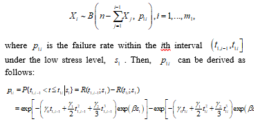

Note that when the baseline function is a simple linear function, we let    Then, we generate    failure times randomly from a uniform distribution within each subinterval   . Therefore, the total number of failure times generated under  is .

Step 2: Generating the number of failures and the failure times under the middle stress level, :

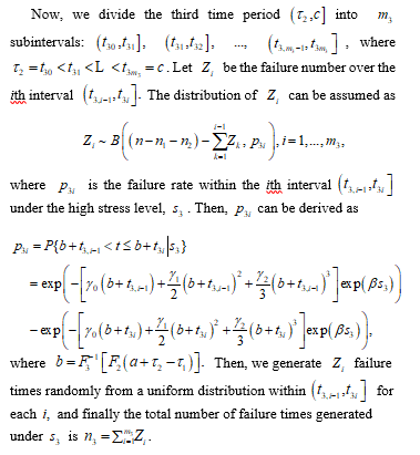
Similarly to Step 1, we divide the second time period  into  subintervals:         , where   Let    be the failure number over the ith interval    the distribution of    can be assumed as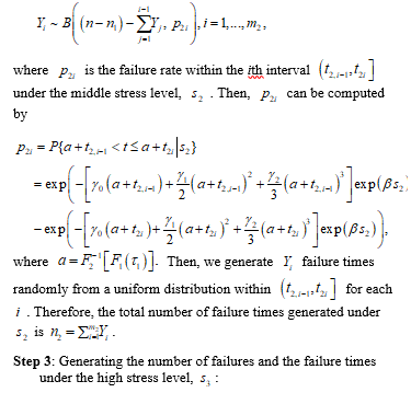

Step 4: Estimating the parameters:

For simplicity, we keep the length of all subinterval equal to    hours in this paper. The log-likelihood function can be expressed as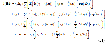

For each simulation run, we can compute the maximum likelihood estimates of the model parameters by maximizing (21).

Let    be the number of simulation runs. We may use these    estimates to calculate the simulated squared bias (SBIAS ), simulated variance (SVAR), and simulated mean squared error (SMSE) of each parameter estimator. We define SBIAS  SVAR, and SMSE for an estimator    as: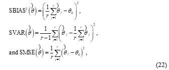

where  is the given true parameter value,  is the estimate of from the jth simulation run. By these definitions, we can compute SBIAS  SVAR, and SMSE respectively for   ,   ,   , and    using the resulting designs from the example obtained in Sections 3 and 4. We can also compute SBIAS  SVAR, and SMSE of the MLE of hazard rate over  under normal design conditions for our resulting designs. The true hazard function over   under normal design stress level  can be expressed as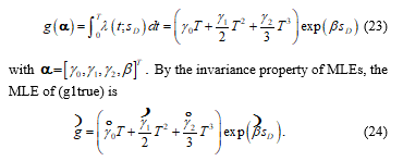

Then, SBIAS  , SVAR, and SMSE of    can also be computed by (22).

5.2.  Performance of the optimal designs obtained in Sections 3 and 4

Taking n = 200,  c = 300 hours, and , the length of all subintervals to be 5 hours, we use the simulation procedure introduced in Section 5.1 to evaluate the performance of our resulting designs. We adopt the constraint case    for a demonstration.

For the PH model with a simple linear baseline function, from Section 3.3, having       , is the D-, A-, and Q-optimal design with fixed middle stress at  . After we update    to the optimal middle stress level, we get new D-, A-, and Q-optimal designs for  . Since the resulting D-, A- and Q-optimal designs are similar, we only present the simulation result for our Q-optimal design. The Q-optimal design we obtained in Section 3.4 for  is    with  ,   ,  . We denote the efficiencies of a design    relative to another design    in terms of SBIAS , SVAR, and SMSE as  , , and  respectively. Based on these  1000 simulation runs, we compute all the SBIAS , SVAR, and SMSE of the MLE for , , , and  when each of the two different designs,  and  , is adopted. Table 13 shows the efficiencies of    relative to    in terms of SBIAS , SVAR, and SMSE of      and (24) respectively. We note that since these are Q-optimal designs and therefore the efficiency gains appear more for estimating  This is consistent with the previous finding of the asymptotic efficiency gains as discussed in Section 3. The simulation results indicate that the most efficiency gains appear in variance reduction with an extreme for . The reason behind is that the optimal designs constructed was aiming to minimize the asymptotic variances.

In Section 3, the Q-optimal designs are obtained by minimizing the asymptotic variance of the . As expected, when  was adopted, we have gained the most efficiency (as high as 76.57%) in terms of the SVAR( ) compare to . The SVAR of MLE of the model parameters are all very much reduced, and their efficiency gains of    relative to    in terms of SVAR( ), SVAR( ), and SVAR( ) are all higher than 100%. Moreover, SBIAS  and SMSE of  are also being reduced. All the results confirm that  outperforms the design

Table 13. The efficiencies of    relative to  in terms of SBIAS , SVAR, and SMSE

	0.9824	0.9803	1.0	1.0175
	2.2207	24508114.61	2.0038	1.7657
	0.9838	0.9851	1.0	1.0345

For the PH model with a quadratic baseline function, the optimal design  having , ,   (please see Table 8) is the D-, A, and Q-optimal designs with a fixed middle stress at . When we simultaneously choose an optimal middle stress together with optimal stress-changing times, the D-, A-, and Q-optimal designs become    having ,  having   and  having   and they all are with  We note that the D-optimal design and Q-optimal design are quite similar. Thus, we only present the simulation results for our resulting A- and Q-optimal designs in this example. Based on the 1000 simulation runs, we compute all SBIAS , SVAR, and SMSE of the MLE for , , ,  and  when each of the three different designs,   , and  is adopted. Tables 14 and 15 display the efficiencies of  and  relative to   in terms of SBIAS , SVAR, and SMSE of ,     ,  and (24) respectively. The simulation results have shown that the designs,  and  by optimally selecting the middle stress level and stress-changing time simultaneously can reduce SVAR( ) by 282% and 183% compared to . We also note that not all of SVARs of MLE of model parameters have been reduced much by using  or . Only SVAR( ) and SVAR( ) have significantly lessened among all SVARs. Further, we uncover that both SBIAS  and SMSE of all , , , ,  and  are reduced by adopting either  or . The efficiencies of    or    in terms of SMSE( )  are more than 50 and 39 times higher than . This indicates that unitizing    or   can provide a great efficiency gain when experimenters are interested in estimating a hazard rate.

Conclusion

Optimal three-step-stress ALT designs for PH models, with either a linear or a quadratic baseline function, have been constructed in this paper. For a three-step-stress ALT, the practitioner often naturally set the average of high and low stress as the middle stress level. Nevertheless, from the results of both simulated and asymptotic efficiency comparison, we have revealed that the optimal three-step-stress ALT designs with both optimal stress-changing times and with an optimal middle stress level outperform the most among all the designs and for all the scenarios considered. Therefore, the three-step-stress plans with both optimal stress-changing times and optimal middle stress level are recommended especially when the hazard rate prediction is interested.

In Section 3, we have presented the resulting optimal designs for a practical ALT example when fitting a PH model with a simple linear baseline hazard function. Taking six different MNF constraint cases, we have found the optimal allocations of the stress-changing times and the optimal middle stress level that can minimize the loss function , , or . Thus, we have solved the minimization problem for a nonlinear objective function with multiple nonlinear constraints (MNF at different stress levels), and obtained the constrained optimal designs under each of D-, A-, and Q-optimality. The resulting optimal designs under three different criteria are quite similar. In addition, we have also found that the middle stress level should be kept as close to the lower bound of the middle stress level as possible as long as the constraint condition is satisfied.

Table 14. The efficiencies of    relative to  in terms of SBIAS , SVAR, and SMSE

	1.0098	21.2561	1.0004	504.6733	313.2065
	0.97136	11.4924	0.0277	420.4643	2.8329
	1.0097	14.0173	1.0004	42.7565	40.2554

In Section 4, we have derived the optimal designs when fitting a PH model with a quadratic baseline hazard function. The optimal stress-changing times and the optimal middle stress level are also chosen in order to minimize the loss functions under given nonlinear constraints. Similarly to the case with a linear baseline hazard, under these constraints, the optimal middle stress level can be located as close to the low stress level as possible as long as such constraints are satisfied. For each of D-, A-, and Q-optimality, six different constrained optimal designs have been obtained. We also reveal that designing a three-step-stress ALT with a fixed middle stress seems only helping reduce the value of loss function under A-optimality. Thus, we suggest not conveniently taking the average of other two stress levels as the middle stress level, especially when a quadratic baseline hazard function is considered. We conclude that optimal three-step-stress designs have gained efficiency on an average of 68% for a hazard rate prediction compared to the corresponding optimal two-step-stress designs, which means that there is 7.56 times higher efficiency gain attained than the case when the baseline function is simple linear.

Table 15. The efficiencies of    relative to   in terms of SBIAS , SVAR, and SMSE

	1.0271	31.4599	1.0004	199.0405	280.6279
	0.7898	6.8388	0.0149	309.2855	3.8197
	1.0258	9.8674	1.0004	29.3142	51.1622

In Section 5, we have evaluated the performance of our resulting designs from both Sections 3 and 4 by simulations. The design for a three-step-stress ALT with an optimal middle stress level and two optimal stress-changing times has greatly increased the simulated efficiency of the hazard rate estimator. It is confirmed that the optimal designs with optimal middle stress significantly outperform those ones with the middle stress level fixed at the average of other two stress levels.

We note that although the design construction in this paper has been demonstrated by optimal designing three-step-stress ALT experiments when a single stress factor is involved, the method developed can be easily extended to conducting the optimal designs for more complicated multiple step-stress ALT, such as step-stress ALT with more than three steps, and/or ALT with multiple stress factors (but one of them engaged in conducting step-stress plans). We also notice that the inaccuracy of the assumed baseline hazard function can cause unavoidable prediction bias. Although the proposed designs perform very well when the model assumed is correct, they seem not helping much in reducing such bias when the assumed model is incorrect. If possible imprecision of the assumed PH model is suspected, then robust design approach should be considered. Some discussion on robust design for a PH model can be seen in [18].

Conflict of Interest

We declare that there is no any conflict of interest.

Acknowledgment

The research is supported by the Natural Sciences and Research Council of Canada.

1.  X. Xu, W. Huang, “Constrained Optimal Designs for Step-stress Accelerated Life Testing Experiments” Proceedings of the 3rd IEEE International Conference on Cloud Computing and Big Data Analysis, 2018, 633-638.
2.  X. Xu, S. Hunt, “Robust Designs of Step-Stress Accelerated Life Testing Experiments for Reliability Prediction” Matematika, 29(1), 203-212, 2013.
3.  R. Miller, W. Nelson, “Optimum Simple Step-Stress Plans for Accelerated Life Testing” IEEE Transactions in Reliability, 32(1), 59-65, 1983.
4.  D. S. Bai, M. S. Kim, S. H. Lee, “Optimum simple step-stress accelerated life tests with censoring” IEEE Transactions in Reliability, 38(5), 528-532, 1989.
5.  D. S. Bai, M. S. Kim, “Optimum simple step-stress accelerated life tests for Weibull distribution and Type-I censoring” Naval Research Logistics, 40(2), 193-210, 1993.
6.  N. Fard, C. Li, “Optimal simple step stress accelerated life test design for reliability prediction” Journal of Statistical Planning and Inference, 139(5), 1799-1808, 2009.
7.  S. Hunt, X. Xu, “Optimal Design for Accelerated Life Testing with Simple Step-Stress Plans” International Journal of Performability Engineering, 8(5), 575-579, 2012.
8.  H. Ma, W. Q. Meeker, “Optimum step-stress accelerated life test plans for log-location-scale distributions” Naval Research Logistics, 55(6), 551-562, 2008.
9.  L. Jiao, “Optimal allocations of stress levels and test units in accelerated life tests,” Ph.D Thesis. Rutgers University-New Brunswick, New Brunswick, New Jersey, 2001.
10.  E. A. Elsayed, H. Zhang, “Design of Optimum Simple Step-Stress Accelerated Life Testing Plans” Proceedings of the 2nd International IE Conference, 1-14, 2004.
11.  C. H. Hu, R. D. Plante, J. Tang, “Step-stress accelerated life tests: a proportional hazards–based non-parametric model” IIE Transactions, 44(9) 754-764, 2012.
12.  N. Becker, B. McDonald, C. Khoo, “Optimal designs for fitting a proportional hazards regression model to data subject to censoring” Austral. J. Statist. 31, 449-468, 1989.
13.  H. Dette, M. Sahm, “Minimax optimal designs in nonlinear regression models” Statist. Sinica, 8, 1249-1264, 1998.
14.  J. M. McGree, J. A. Eccleston, “Investigating design for survival models” Metrika, 72, 295-311, 2010.
15.  J. L´opez-Fidalgo, M. J. Rivas-L´opez, R. Del Campo, “Optimal designs for Cox regression” Statistica Neerlandica 63, 135-148, 2009.
16.  M. Konstantinou, S. Biedermann, A. Kimber, “Optimal designs for two-parameter nonlinear models with application to survival models” Statistica Sinica, 24, 415-428, 2014.
17.  W. Nelson, Accelerated Testing: Statistical Models, Test Plans, and Data Analyses. Wiley. New York, 2004.
18.  X. Xu, W. Huang, “Optimal Robust Designs for Step-stress Accelerated Life Testing Experiments for Proportional Hazards Models” Mathematical and Computational Approaches in Advancing Modern Science and Engineering, Eds: Bélair, J., Frigaard, I.A., Kunze, H., Makarov, R., Melnik, R., Spiteri, R.J., New York: Springer, 585-594, 2016.

(Click Here)

(Click Here)