1. Introduction

This paper is an extension of a work originally presented in the 2018 Joint IEEE EMC & APEMC, which took place in Singapore from 14 to 17 May 2018 [1], and its main purpose is to present in a more detailed form both the general theoretical framework and the demonstration that the circuit’s theory applies to the two degrees of freedom of the so-called longitudinal mode: the scalar potential “Ф” in the conductor and the magnetic potential “A_mz” along the conductor (the current “i” in the conductor is related to A_mz through the concept of inductance).

In reference [1], this theory was applied to study conducted and radiated interferences in transmission lines, because there exists confusion among the people that work in the area, in different time scales; which is caused, as mentioned there, by a rather loose definition of conducted and radiated disturbances.

But nor the answer to the question, why do we feel that they are rather loosely defined? was fully explained in the text of reference [1], neither the primary cause of the confusion was identified.

In reference [1] it was recalled that “in IEC, the disturbing electromagnetic fields are divided into: conducted disturbances (IEV 161-03-27) and radiated disturbances (IEV 161-03-28).

The essential difference between these disturbances, as established in the above definitions, resides in the manner how the energy is transferred to the conductors:

– For conducted disturbances, IEV 161-03-27 says that the energy is transferred via one or more conductors;

– For radiated disturbances, IEV 161-03-28 says that the energy is transferred through space in the form of electromagnetic waves. However, it notes that “The term “radiated disturbance” is sometimes used to cover induction phenomena”.”

We feel that the above definitions of conducted and radiated disturbances are rather loosely defined because they appeal to an intuitive concept of energy on the part of the reader, taking advantage of the fact that the electromagnetic energy is very seldom calculated in interference problems. Besides that, the concept of electromagnetic energy of the people that works in circuit terms is very different than the concept of the people that works in field terms.

IEV definition of electromagnetic energy 121-11-64 says that “The energy associated with an electromagnetic field, in a linear medium within a domain V, is given by the volume integral

where E, D, H and B are the four vector quantities determining the electromagnetic field”.

This definition in field terms is not easy to understand for the people working in the low-frequency regime, which is used to work in circuit terms. Also, it is not frequently known what the relation between the above defined concept of electromagnetic energy and the concept of energy and power, used in circuit terms, is.

Then, we can trace back the primary cause of the confusion to the fact that some people work in circuit terms, while other people work in field terms.

As mentioned in reference [1], this is the origin of the different approach and the rather different language used by the people working in the low-frequency regime, as the power quality area, and the people working in the high-frequency regime, both in the lightning protection area and in the EMC area, facts that cause a certain degree of confusion and make it difficult the communication among the people working in these different areas.

Also, as very well observed in reference [2], “Within IEC, power quality is treated within the standards on electromagnetic compatibility (EMC)”. This is because EMI problems, both in the low-frequency regime and in the high-frequency regime, are quantified and measured in terms of currents in the conductors and voltages between conductors, which is partly due to the widely accepted belief that the EMI on transmission lines is a completely known problem, and it can be simulated using various circuit simulation software’s.

But this belief assumes that the problem of determining to what kind of electromagnetic systems the circuit theory is applicable, or which are the limits of the validity of the circuit theory, is a solved problem. Assumption that is by no means valid [3].

In this paper, as in reference [1], we first demonstrate that the characterization of the electromagnetic field in terms of the electric scalar potential “Ф” and of the magnetic vector potential “A_m” [4], which Maxwell called electromagnetic momentum [5], when the matter can be macroscopically described by constitutive laws, is totally general. This characterization has in total four degrees of freedom.

Second, we demonstrate that the circuit’s theory applies to the two degrees of freedom of the so-called longitudinal mode: the scalar potential “Ф” in the conductor and the magnetic potential “A_mz” along the conductor (the current “i” in the conductor is related to A_mz through the concept of inductance).

This paper is organized as follows:

In part 2, which closely follows the description given in part II of reference [1], we first review the different forms of description of the electromagnetic field within the matter [4, 6-9] showing that all of them have in common the equations involving the vector fields E (electric field strength) and B_m (magnetic flux density), which are commonly called “electric field” and “magnetic field”.

Also, as in reference [1], it is shown that:

– When the matter can be macroscopically described by constitutive laws, which are relations between the other fields (H, D and J_efr) needed to describe the electromagnetic field within the matter and the fields E and B_m; then, the electromagnetic field within the matter is fully characterized by the fields E and B_m (six degrees of freedom); and

– As the common equations for the fields E and B_m can be solved in terms of the so-called magnetic vector potential “A_m” and electric scalar potential “Ф”, in the case when the matter is described by constitutive laws, the number of degrees of freedom needed for the characterization of the electromagnetic field within the matter can be reduced from six (E, B_m) to four (A_m, Ф).

Then, as it happens in the vacuum [10], when the matter is macroscopically described by constitutive laws, the electromagnetic field within the matter is fully described by these two potential fields A_m and Ф.

The extension made in this paper mainly refers to alert the reader on the differences, arising from the different formulations of electromagnetic theory and not always acknowledged, between the formulations utilized by the different application software’s.

In part 3, which closely follows the line of reasoning of part III of reference [1], we first show that when the matter is predominantly distributed along a certain direction in space, as for transmission lines, the four degrees of freedom of the potentials can be separated into two independent modes, each of them with two degrees of freedom:

– a longitudinal mode constituted by Ф and the component of A_m along the line, which is a TM (transverse magnetic) mode [11], and

– a transversal mode constituted by the two components of A_m transversal to the line, which is a TE (transverse electric) mode [11].

As in reference [1], it is also shown that the longitudinal mode is the one described by circuit theory and the relation between its two degrees of freedom is given by Kirchhoff’s laws, which are deeply related to the existence and predominance of the longitudinal mode.

As an extension made in this paper, using the longitudinal TM mode as the fundamental building block, instead of the TEM (transverse electromagnetic) mode as in traditional transmission-line theory [12], and assuming that the longitudinal and the transversal modes are practically independent, we present the derivation of a generalized theory of the electromagnetic field coupling to a multiconductor line, in time domain, that, as usual, predicts the propagation of the scalar potential and the current along the line.

For the longitudinal TM mode, as in traditional multi-conductor transmission-line theory [12-14], the line voltages have a unique value, independent of the integration path from the reference to the conductor.

The independent transversal mode produces additional induced voltages (integration path dependent) between the conductors of the line.

As mentioned in reference [1], this treatment can also be extended to lines with imperfections, discontinuities or with conductors attached perpendicular to the line, such as, the terminations, equipment connections or groundings [15].

Also, as an extension and an application of the concept of longitudinal mode, the derivation of a general theory of the coupling of an external electromagnetic field to a conductor line is presented. This theory can be applied to different problems, such as, electromagnetic neural stimulation [16-20] and the calculation of lightning-induced voltages [13]. In order to not deviate the attention away from the main purpose of the paper and to avoid too many mathematical derivations in the main body of the paper, we present it in Annex 1.

The generalized theory of the electromagnetic field coupling to a multiconductor line, under the proper simplifications, reduces to the standard coupling theories [12-14,21]. In Annex 2, we present a detailed comparison of this generalized theory with the most important classical theories of the electromagnetic field coupling to a multiconductor line.

In part 4, as in part IV of reference [1], we apply the above theory to analyze the interference on a transmission line produced by external disturbances, which are commonly classified into conducted and radiated disturbances.

As in reference [1]:

– We assume that the normal operation mode, which is driven by normal lumped external excitation sources, is a longitudinal mode;

– We divide the externally produced disturbances in two classes: longitudinal mode disturbances and transversal mode disturbances;

– We divide the longitudinal mode disturbances in two classes: the scattered and the externally produced; these last ones are also divided in two classes: the remotely produced and that produced by the impressed current, which is injected by lumped external sources.

We show that:

– the conducted disturbances are longitudinal mode disturbances that affect only the longitudinal mode; but,

– the radiated disturbances are composed of longitudinal mode disturbances and transversal mode disturbances, both of which affect the longitudinal mode; while the transversal mode is only affected by the transversal mode disturbances.

This is the reason why, only when the longitudinal and the transversal modes are practically decoupled, EMI can be simulated using circuit simulation software’s.

Also, this explains why current injection and capacitive clamp testing methods represent only the effect of disturbances, both conducted and radiated, on the longitudinal mode.

In part 5, in order to illustrate the interpretation power of this approach, we present the results of other application cases together the important practical and engineering conclusions that has gone unnoticed in other calculations made with previously proposed approaches/software tools. Finally, in part 6 we present our summary and our main conclusions.

2. Description of the Electromagnetic Field

The description of the electromagnetic field given in this paper closely parallels the description given in reference [1] having only being added some complementary explanations, being (1) to (8) the same of reference [1] and our (13) is equal to (9) of reference [1].

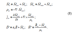
The Maxwell-Hertz classical formulation of the electromagnetic theory [4,6], which refers to 5 vector fields and 1 scalar field (E, H, D, B_m, J_efr and ρ_efr), is commonly called Maxwell equations (IEV 121-11-62):

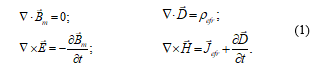Where the four quantities determining the electromagnetic field (IEV 121-11-61) are: E the electric field strength (IEV 121-11-18), H the magnetic field strength (IEV 121-11-56), B_m the magnetic flux density (IEV 121-11-19) and D the displacement (IEV 121-11-40). The vector field J_efr is the electric (conduction) current density (IEV 121-11-11) and the scalar field ρ_efr is the electric charge density or volumic (electric) charge (IEV 121-11-07), which according to IEV 121-11-61 are needed to characterize the electric and magnetic conditions of a material medium together the electromagnetic field.

 Using the following definitions:

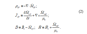Where: M_efr and M_mfr are the electric and magnetic matter fields produced by the free electric charges; B_e, which is called the electric flux density, is a vector field composed of D and M_efr.; and H_e, which is called the magnetic field intensity, is a part of the vector field H that is composed of H_e and M_mfr.

Then, (1) can be written in a more symmetrical form [7] as:

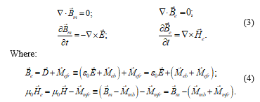M_eb and M_mb are the electric and magnetic matter fields produced by the bound charges.

It is important to note that our definition of electric flux density B_e is different from the definition of IEV 121-11-40, where they call “electric flux density” to the displacement D (saying that this last terminology is obsolete), despite not being divergence-less. Also, our definition of magnetic field intensity H_e is different from the definition of H, the magnetic field strength of IEV 121-11-56.

Equations (3) constitute the formulation of the electromagnetic theory that is called “Symmetrical theory of electromagnetism” [7].

The two vector equations in (3) can be interpreted as state equations, with the flux fields B_e and B_m representing the electric state and the magnetic state, respectively; and the intensity fields (E and H_e) being the necessary inputs to produce a change in the states.

Using (4), (1) and (3) can be written as:

From (5) and (6) it is clearly seen that the sources of E and B_m are M_e and M_n. Equations (5) constitute the Feynman’s formulation of the electromagnetic theory [8].

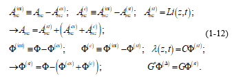
If instead of separating the matter fields M_e and M_n into fields produced by free and bound charges, as in (6), we make the separation of the matter fields into fields produced by charges that are internal (M_ei and M_mi) or external (M_eex and M_mex) to the piece of matter considered; then we have:

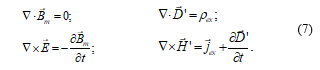
Equations (7) constitute the Landau & Lifshitz’s formulation of the electromagnetic theory [9].

All the usual formulations of the electromagnetic theory, as (1), (3), (5) or (7), have in common the equations of the left-hand side involving the vector fields E and B_m.

Usually, these left-hand side equations are solved in terms of the so-called magnetic vector potential “A_m” and electric scalar potential “Ф”:

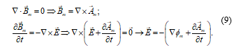In most electromagnetic theories, the potentials have not physical reality, then the divergent of the magnetic potential can be arbitrarily chosen. The most common choices are:

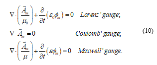In the “Symmetrical theory of electromagnetism” [7], there exist potentials that have physical reality, which are those related to the Hertz’ potentials, which fulfill the following restriction:

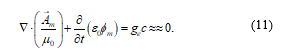Saying that the Lorenz’ gauge has physical reality. However, as in the normal Lorenz’ gauge, there exist a manifold of magnetic potentials that are mathematically equivalent to the real potentials, in the sense that they produce the same magnetic flux density and the same electric field strength, which are the quantities that are universally recognized as having physical reality. These are:

In the macroscopic formulation of the electromagnetic theory, usually the vector fields appearing in the right-hand side of (1), (3), (5) or (7) are expressed in terms of the fields E and B_m, by means of the so-called constitutive laws.

For example, for the Maxwell-Hertz’s formulation (see (1)), we have:

The parameters “σ”, “ε” and “μ”, appearing in (13), are called electric conductivity, electric permittivity and magnetic permeability, respectively.

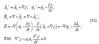
Then, (1) can be written in terms of the potentials as:

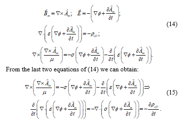
The last two equations of (14) are four scalar equations to determine the components of the four-vector formed by “A_m” and “Ф/c” [10], which we will call “A_em”, whose source is the free electric charge density. Equations (15) says that for a conduction dominated medium the real source is the time variation of the free electric charge density.

Then, in the case where the matter is described via constitutive laws, the field “A_em”, with only four degrees of freedom, fully describes the electromagnetic field.

This is the formulation applied in [22].

When dealing with interference problems is very important to distinguish what belongs to the system being studied and what is considered an externally applied electromagnetic field.

Then, we will write the equations corresponding to (13) and (14) for the Landau & Lifshitz’s formulation (see (7)), which makes this separation. In this case we have:

The parameters “σ*”, “ε” and “μ*”, appearing in (16), are also called electric conductivity, electric permittivity and magnetic permeability, respectively.

Then, (7) can be written as:

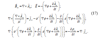Again, the last two equations of (17) are four scalar equations to determine the components of the four-vector “A_em”, formed by “A_m” and “Ф/c”, whose sources are the external electric charge density and the external current density. Then, also in this case the field “A_em”, with only four degrees of freedom, fully describes the electromagnetic field.

We can write the last two equations of (17) in a different manner:

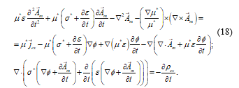Equations (18) show that, in the case of the electromagnetic field within the matter, even in the Maxwell’s gauge, in general, the equations for ϕ and A_m are not separable, as in the case of the vacuum. Besides that, the simple retarded solutions are not applicable.

For the special case of time-harmonic electromagnetic fields, or in frequency domain, (17) is simplified, by the fact that we can express the external charge density in terms of the divergence of the current density, and for the last two equations of (17) we have:

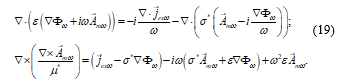Equations (19) show clearly that the sources of the induced electromagnetic field are the external electric charge density and the external current density.

This is the formulation applied in [23,24].

3. Transmission-Lines

As in reference [1], and our (20) to (24) are the same than (11) to (15) of reference [1], in the case of the transmission lines, matter is predominantly distributed along a certain direction in space, which we will call it “z”, making this a preferential direction.

As the four-dimensional vector field “A_em” transforms as a four-vector [10], for a transformation of coordinates between a system moving with a velocity “v”, along the preferential z-axis, relative to another “rest” system, which we denote by the index “0”, we have:

From (20) we can see that, for horizontal (along the z-axis) ideal transmission lines (having an uniform cross section), we can divide the electromagnetic field into two independent modes, each one with two degrees of freedom: a first one composed of “Ф” and “A_mz”, which will be called longitudinal mode; and a second one composed of “A_mx” and “A_my”, which will be called transversal mode.

Transmission lines constituted of insulated filamentary conductors, disposed along the z-axis, can internally produce only the longitudinal mode. The transversal mode must be externally produced.

The transversal mode can only be internally produced if the transversal extension of the conductive matter is relevant or if the filamentary conductors are not insulated.

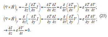
For the longitudinal mode (A_mx = A_my = 0), from the first two equations of (11) or (14), we have:

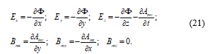Equations (21) say that the longitudinal mode is a TM mode, and, that the transversal electric field is conservative and is equal to the transversal gradient of the scalar potential Ф. This allows the definition of transverse voltages that are single valued [11, 12, 14].

For the transversal mode (Ф = A_mz = 0), we have:

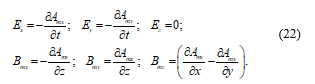Equations (22) say that the transversal mode is a TE mode, with a non-conservative transversal electric field.

As an example of a pure longitudinal mode, we will see first the special case treated by Schelkunoff [11], of an infinite horizontal hollow conductor of arbitrary cross-section, rigid and made of perfectly conducting matter. Here, if we can assume that “Ф” and “A_mz” are separable, we have:

Where, in equations (23) the T functions are dimensionless functions of x and y.

Using (23) in (21), we have the Schelkunoff’s TM modes [11]:

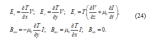Also, from the equations on the right-hand side of (1) and (3), we have:

Equations (24) and (25) display the main characteristic of Schelkunoff’s TM modes, which is the fact that, even in the case of a hollow conductor made of perfectly conducting matter, despite having an electric field strength value equal to zero within the conductor, there can be an electromagnetic field inside the conductor, which propagates along the z axis, following transmission-line equations. The existence of this longitudinal mode and its predominance, even for hollow conductors that are slowly bent, leads to the theory of waveguides.

The other very important special case, where the longitudinal mode is predominant, is the case of a multi-conductor transmission line having, in general, many (N+1) filamentary conductors.

Here, following the same line of reasoning and adopting the terminology utilized in reference [1], we will describe the interaction of an arbitrary external electromagnetic field with a straight segment of a multiconductor line.

In Annex 1 the case of an elementary single-wire line is treated in detail. There we present the derivation of a general theory of the coupling of an external electromagnetic field to a conductor line and a detailed comparison of this generalized theory with the most important classical theories. This theory can be applied to different problems, such as, electromagnetic neural stimulation [16-20], the calculation of lightning-induced voltages [13].

In the case of a multiconductor line, we can obtain from (9) or (21) the value of the longitudinal electric field strength, at a point internal to the “j” conductor (see Figure 1), for j = 0 … N:

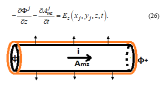Figure 1 – Segment of a conductor, of length “Dz”, between two scalar potential nodes.

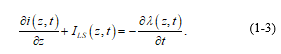
Also, integrating the divergence of the last equation of (14) in a closed surface that involves a segment of length “Dz” of the horizontal “j” conductor (see Figure 2), we have:

      Where, “i^j” is the total current flowing through the cross-section of the “j” conductor, “l^j” is the charge accumulated on the surface of the “j” conductor, per unit length, and “I_LS^j” is the conduction current flowing out of the “j” conductor through the lateral surface, per unit length.

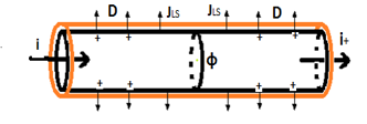Figure 2 – Segment of a conductor, of length “Dz”, around a scalar potential node.

If, as usual, we assume that for this kind of transmission line, for which the distances among the different conductors of the line is much shorter than its length, the Maxwell’s concept of inductance and capacitance coefficients are valid [25,26].

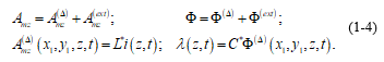
This will allow us to express the magnetic potential in a short segment of a filamentary conductor, at a point “z” along the line, in terms of the current in all the conductors at the same point “z”, and, the charge at the surface of a conductor, at a point “z”, in terms of the scalar potential at all the conductors at the same point “z”. Then, we have:

Where: “A_mz^j(Δ)” and “Ф ^j(Δ)” are the potentials produced by the matter existing in all the conductors within the segment “Dz”, at the point “z”; and “A_mz^j(ext)” and “Ф ^j(ext)”, are the potentials produced by the matter existing in all the conductors, outside the segment “Dz”, plus the potentials “A_mz^j(ex)” and “Ф ^j(ex)” representing the externally applied field.

Using Ohm’s law for the line conductors, we have:

Where “R_(cj)” is the resistance, per unit length, of the conductor “j”.

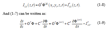
Extracting from the conduction current “I_LS^j”, flowing out of the conductor through the lateral surface, the part that is due to the linear leakage current, we can write:

Then, (26) and (27) can be written as:

Where: “[L*]”, is the matrix of the inductance coefficients, per unit length; “[C*]” is the matrix of the capacitance coefficients, per unit length; and “[G*]” is the matrix of conductance coefficients, per unit length, between the segments of all conductors at the point “z”.

To describe a rectilinear transmission line of a uniform cross-section and of a finite length, we can use here again, as usual in transmission-line theory [12], the matrices [L], [C] and [G], which are calculated neglecting the retardation effects and when every conductor of the line is uniformly charged with a charge density, per unit length, which is equal to its value at the point “z”, and the current in all segments along the line, in any conductor, is equal to its value at the point “z”. The potentials produced in this situation are the static potentials “A_mz^(st)” and “Ф ^(st)”. Using for every conductor “j” the following definitions, we have:

Where the usual summation rule over repeated index is applied.

Then, we can write (31) and (32) as:

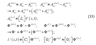
As mentioned in reference [1], “the main variables in (34) and (35) are the scalar and the magnetic potentials, which are not uniquely determined (see (12)). Their values, as well as the value of the inductance and capacitance coefficients, are affected by the choice of the reference point, which is the point where the value of the potentials is equal to zero.

But, as the fields E and B_m are uniquely determined and, for practical purposes, the important voltages are the ones occurring between the conductors of the line, this fact is of little or no importance.”

We will choose the reference for the potentials at the infinity, or at a line located very far from the multiconductor transmission line.

With this choice of reference, (34) can be interpreted as the application of Kirchhoff’s circuits law applied to a “mesh” formed by a segment of the conductor “j” of the line and the reference line; and (35) as the application of Kirchhoff’s circuits law applied to a potential node on the conductor “j” of the line. Then, we can see that the longitudinal TM mode is the one described by circuit theory.

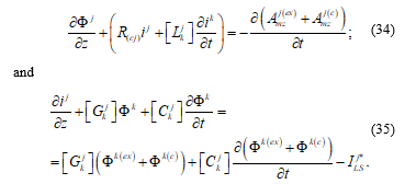
Also, (34) and (35) are completely general and rigorous equations that describe the interaction of an external electromagnetic field with the considered filamentary multi-conductor transmission line, being the only assumptions in deriving these equations: the thin-wire approximation for all the conductors and the validity of Ohm’s law for all the conductors. Thus, they constitute a generalized formulation of the electromagnetic coupling to a transmission line that, under the proper simplifications, reduces to the standard coupling theories [12-14,21] (see Annex 2).

One of the advantages of the time domain formulation of the longitudinal mode is that (34) and (35) can also be written as state equations:

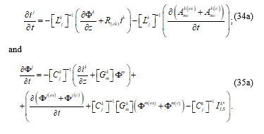Then, (34a) and (35a), which are a generalization of (21a) and (22a) of reference [1], as already mentioned in reference [1], “can be interpreted as saying that the scalar potential “Ф^j” and the current “i^j” represent the time evolving state of the system, at a point internal to the “j” conductor.” Showing that the essence of the circuit theory is to assume that the longitudinal mode is predominant.

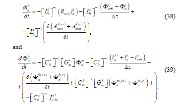
Equations (34a) and (35a), after being spatially discretized into N segments (for n = 1…N), can be written as:

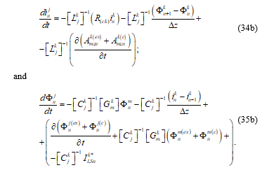Equations (34b) and (35b), as also mentioned in reference [1], “are a system of coupled ordinary differential equations (ODE), for the scalar potential at potential nodes and the current at current nodes.” Also, as already mentioned in reference [15], “this system of coupled ordinary differential equations can then be solved using the powerful ODE solvers now existing” [27].

The main advantage of describing uniform lines by per-unit length parameters, calculated using the static potentials is that these parameters are constant and easy to calculate, particularly, when the reference is taken at the infinity, because it is a reference independent of the direction of the line.

For obtaining approximate solutions of non-uniform lines, assuming that the longitudinal mode is predominant, the non-uniform line is usually modeled as a cascade of uniform sections, conductively connected [28]; or in the case of lines with periodically varying cross-section, such as the cables composed of twisted-wire pairs, the line is modeled as an equivalent line, having per-unit length parameters equal to the average over the period [29].

Up to now, we have studied the uniform or slowly non-uniform part of the line.

As mentioned in reference [1], using reference [15], “we will take advantage of this formulation that allows to include the interaction of a segment of conductor with any known arbitrary external electromagnetic field, which can be described by Ф^(ex) and A^(ex), to include the terminations of the line, the discontinuities or even conductors attached perpendicular to the line, such as, groundings or other equipment connected.”.

Considering that the longitudinal mode is predominant, we can model them as circuit elements located between two potential nodes, which are displaced in space along a certain direction.

For a vertical conductor (y axis direction) that is relatively small (compared to the minimum wavelength of interest), so that we can neglect the corrections due to the time delay in the production of the potentials, and neglecting also the non-linear transversal conduction current I_LS^*, we have in a manner analogous to (31) and (32):

This is the explanation of the important remark quoted in the conclusions of reference [14] “When using the scattered-voltage formulation, it must be remembered that the vertical component of the incident electric field appears as a voltage source in the line terminations.”

If, like in the case of a grounding of the reference conductor, the vertical conductor is connected at the potential node “Ф_n⁰”, the modified equations for this node are:

Where, in this case, only “i_n⁰¹”, which is the current in the first segment of the vertical conductor, is different from zero.

As mentioned in reference [1], “this formulation allows representing the groundings not as a connection to the ground, but as a connection to the grounding electrodes, whose potential is to be considered as one of the states of the system.

This is very convenient for the real cases where the ground is not perfectly conducting, and it is considered as the return conductor of the line.”.

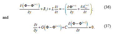
Finally, as in reference [1], to include the effect of the transversal mode, we will define the so-called conductor voltages.

Usually, in standard transmission-line theory, the conductor voltages are defined relative to one of the conductors chosen to be the reference [12, 30]. This was the choice indirectly adopted in reference [1].

Here, we will define the conductor “j” voltage, at a point “z” along the conductor, as the integral of the transversal electric field strength “E_t” between the conductor “j” and the reference of the potentials:

Where we will assume that “A_mt” is the externally produced field, but, as mentioned in reference [1], “the formulation also allows to include the transversal field produced by transversal conductors.”. Then, we can modify (34) and (35), by means of (40), and obtain:

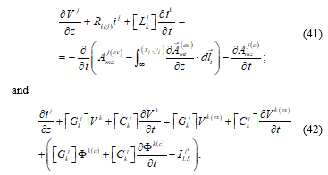Where, as mentioned in reference [1], “we can see that writing the equations in terms of the conductor voltages produce new terms in (41) and (42), due to the existence of induced voltages (integration path dependent) produced by the external transversal mode.”

For the special case of time-harmonic electromagnetic fields, or in frequency domain, (41) and (42) can be written as:

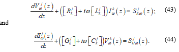
Which, without the sources, are the standard transmission-line equations in frequency domain, such as shown in (2) of reference [30] or (6.7) and (6.8) of reference [31].

As already mentioned in reference [1], “we must note that, for the longitudinal mode, the important values of the externally produced field are at points located inside the conductors, and its effect can be represented as a voltage or a current source; while, for the transversal mode, the important values of the externally produced field are at points located in the dielectric between the conductors, and its effect is to produce an induced voltage between the conductors.”.

Also, as mentioned in reference [1], “it must be emphasized that, in order to define the concept of voltage associated with one point of the line, it is necessary to introduce a reference.

When the reference is at the infinity, or in the case of an imperfectly conducting Earth where the “Reference perfect conductor plane” is located at a remote position within the Earth, both the conductor “j” voltage and the scalar potential of the “j” conductor, will have embedded the complexities of the electromagnetic field distribution in the ground.

Calculate the electromagnetic field distribution within the Earth is a very difficult task, but fortunately, the voltages and the potential differences between aerial conductors, which are the ones of practical importance, will not depend directly on those complexities.”.

4. Interferences produced by external Disturbances

In this part, as in part IV of reference [1], we will apply the generalized theory of the electromagnetic coupling to a transmission line, developed in part 3, to analyze the interference on a transmission line produced by external disturbances, which are commonly classified into conducted and radiated disturbances.

To study the interference due to an external disturbance, we must first separate the sources of the externally produced electromagnetic fields in two classes: the normal external sources and the disturbing external sources.

In the interconnections, which are multiconductor transmission lines, the dominant mode is the longitudinal mode, and, the longitudinal and the transversal modes are practically decoupled.

Then, as in reference [1], we will assume that the normal operation mode, which is driven by normal lumped external excitation sources, is a longitudinal mode.

IEV 161-03-27 says, for conducted disturbances, that the energy is transferred via one or more conductors. So, conducted disturbances are locally produced.

IEV 161-03-28 says, for radiated disturbances, that the energy is transferred through space in the form of electromagnetic waves; and, it notes that “The term “radiated disturbance” is sometimes used to cover induction phenomena”. Then, radiated disturbances are always remotely produced.

Here, as in reference [1], “we will divide the externally produced disturbances in two classes: the first class that produce Ф and A_mz, which will be called longitudinal mode disturbances; and the second class that produce A_mx and A_my, which will be called transversal mode disturbances.”

 Also, as in reference [1], within the internally-produced longitudinal mode, “Ф ^(int)” and “A_mz^(int)”, we must make a distinction between the scattered part and the part that is produced by the current that is injected by lumped external sources, both normal and disturbing.

Then, we have:

Where: the index “N” indicates normal, the index “D” indicates disturbing and the index “exinj” indicates produced by the lumped external sources, conductively connected to the line, that injects current in the line. Our (45) is equal to (33) of reference [1].

In this paper, neglecting the internally-produced transversal magnetic potential, which is produced by the current in the transversal conductors and the transversal leakage currents, we have assumed, as in reference [1], that the transversal mode is produced only by the radiated disturbances.

As mentioned in reference [1], the effect of the transversal mode is:

– to produce an induced voltage between the conductors, and

 – to act as a lumped voltage source located at the transversal conductors, such as the line terminations and groundings.

Then:

– The so-called “conducted disturbances” (IEV 161-03-27) are characterized by the fields Ф^(exinjD) and A_mz^(exinjD), which are produced by a current locally injected into the line, by lumped disturbing external sources conductively connected to it; and

– The so-called “radiated disturbances” (IEV 161-03-28) are characterized by the fields Ф^(ex), A_mz^(ex), A_mx^(ex) and A_my^(ex), which are produced by remotely located sources.

 The confusing note existing in IEV 161-03-28 that “The term “radiated disturbance” is sometimes used to cover induction phenomena”, can be explained because the electromagnetic field, produced by remotely located sources, includes both the induction field and the radiation field:

Where: the index “ind” indicates induction field, which is negligible in the far field region, and the index “rad” indicates radiation field.

From equations (45) we can see that:

1- The conducted disturbances, “Ф^(exinjD)” and “A_mz^(exinjD)”, which produce scalar potentials and inject currents into the line, are longitudinal mode disturbances that affect only the longitudinal mode; while

2- The radiated disturbances, which are composed of longitudinal mode disturbances, Ф^(ex) and A_mz^(ex), and transversal mode disturbances, A_mx^(ex) and A_my^(ex), affect:

–  The longitudinal mode, directly by the longitudinal mode disturbances through the scalar potential “Ф^(ex)” and the magnetic potential “A_mz^(ex)” along the conductors; and indirectly by the transversal mode disturbances through the lumped voltage sources at the transversal conductors and terminations, which represent the effect of “A_mt^(ex)” along the transversal conductors;

 – The transversal mode, through the magnetic potentials A_mx^(ex) and A_my^(ex), which produce an induced voltage between the conductors.

This is the reason why, only when the longitudinal is predominant, and, the longitudinal and the transversal modes are practically decoupled, EMI can be simulated using circuit simulation software’s.

Also, this explains why current injection and capacitive clamp testing methods represent only the effect of disturbances on the longitudinal mode.

Examples of radiated disturbances, where the longitudinal mode disturbances are dominant, can be seen in references [14,21,32], which deal with lightning-induced voltages; and in reference [33], which deal with voltages induced in twisted-wire pairs by a parallel wire excited by a voltage source.

Examples of radiated disturbances, where the transversal mode disturbances are important can be seen in:

– reference [14], where the exciting source is a lumped voltage source, which represents the induced voltage produced by the transversal mode disturbance, along a transversal conductor at input terminal of the line;

– reference [34], where the induced voltage, produced by the transverse mode disturbance, is an important part of the total voltage, and even the dominant part for the first three microseconds.

In reference [2], the conducted disturbances are defined as “Any deviation from the ideal voltage or current waveform”, meaning the presence of a disturbing scalar potential or a longitudinal magnetic potential produced by the current, which is locally injected by lumped disturbing external sources.

Examples of common types and new types of power quality disturbances can be seen in reference [2].

5. Application Case Results

To show the usefulness of this formulation, we present, as in reference [1], the results of some application cases to real transmission lines with transversal conductors, which are connected to the earthing electrodes, in the case of a real ground that is not a perfect conductor. Adding here, in order to show the interpretation power of this formulation, some important practical and engineering conclusions that had gone unnoticed in other calculations made with previously proposed approaches/software tools.

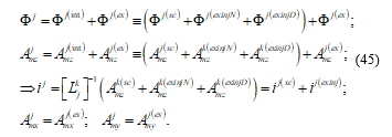
Firstly, as in reference [1], we present in Figure 3 that corresponds to Figure 1 of reference [1], the results of the calculation of the phase-to-neutral voltage, induced by a vertical return stroke that strikes close to a line, which have a neutral wire grounded at only one point, with a grounding resistance of 100 Ω.

As mentioned in reference [1], the purpose of this example is to show that, in this case, the impinging electromagnetic pulse, composed of both a longitudinal mode disturbance and a transversal mode disturbance, initially practically produces only common mode on the line, and, the phase-to-neutral voltage is negligible until the instant when the electromagnetic disturbance reaches the grounding conductor of the neutral wire.

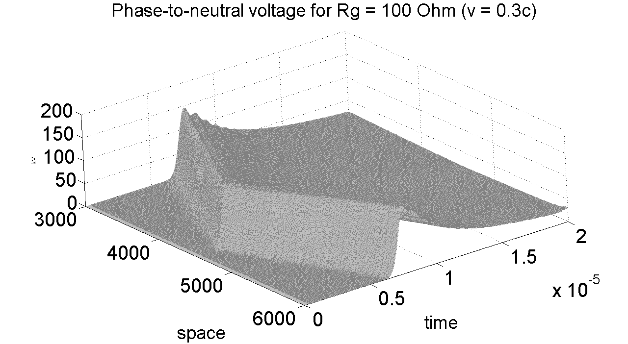Figure 3 – Phase-to-neutral voltage induced by a 100 kA (2×40 ms) return stroke, with velocity 0.3c, which strikes at z = 4000 m, at 100 m from a line, with a neutral wire having an isolated grounding at z = 4500 m, with Rg = 100 Ω. Data taken from [15]

Then, due to the presence of the transversal grounding conductor of the neutral wire, when the electromagnetic transversal mode disturbance reaches the grounding conductor, the current produced by the impinging electric field along the conductor generates voltage reduction waves, which are different in size in the different conductors, thus producing a phase-to-neutral voltage pulse, which propagates in both directions along the line, representing the conversion of common mode into differential mode.

This effect that had gone unnoticed in other calculations made with previously proposed approaches/software tools [15,35], has the important engineering conclusion that the main mitigating effect for the induced voltages is not produced by the shielding wire acting as an extended protective device but by the shielding wire grounding acting as a localized protective device.

As a second example, we present in Figure 4 that corresponds to Figure 2 of reference [1], the results of the calculation of the phase-to-neutral voltage, induced by a vertical return stroke that strikes close to a line, having a neutral wire that is periodically grounded.

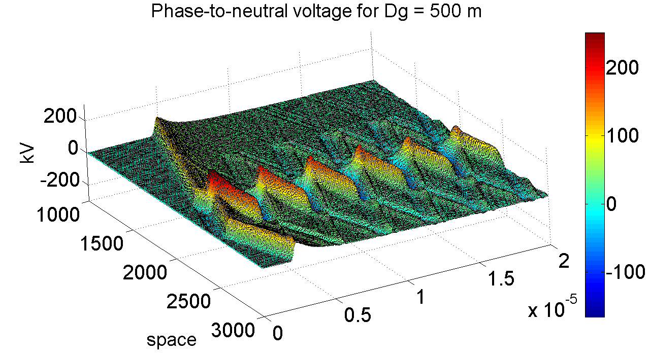Figure 4 – Phase-to-neutral voltage, in a line periodically grounded each 500 m (Rg = 10 Ohms), produced by a 30kA return stroke (0.3×40 ms), occurring at z=2375 m, 50 m from the line. Data taken from [15].

From Figure 4 it can be seen, as already observed in Figure 3, that the impinging electromagnetic pulse produces initially only a common mode perturbation on the line, which propagates in both directions starting from the point of the line which is closest to the stroke location, and the phase-to-neutral voltage is negligible until the instant when the electromagnetic disturbance reaches a transversal grounding conductor of the neutral wire. Then, a phase-to-neutral voltage pulse is produced, due to the injection of current in the transversal wire, which propagates in both directions along the line.

In this case, the effect of the presence of the transversal periodic grounding conductors is to confine the bigger phase-to-neutral overvoltage in the region of the line which is closest to the return stroke location.

Also in this case, the calculations pointed to an effect, which had gone unnoticed in other calculations made with previously proposed approaches/software tools [36], that the presence of the grounding reduces the overvoltage at its location and behind it (seen from the return stroke location), and also it reduces the overvoltage in front of it, but only within a certain distance, fact which defines an “effective distance”.

Then, as mentioned in reference [15], “the shielding wire groundings not only do not protect the line span in front of the return stroke location, but they also produce big positive phase-to-neutral overvoltage”.

In the next example, we present in Figure 5 that corresponds to Figure 3 of reference [1], the results of the calculation of the voltage induced on the conductors of a line, by a vertical return stroke that strikes close to a line, having surge arresters placed periodically on one of the conductors.

From Figure 5, we can see that the effect of the presence of the transversal surge arresters, with its grounding conductors, is:

– On the conductor with surge arresters, to confine the phase-to-reference ground overvoltage, which is oscillating, in the region of the line close to the return stroke location, being the bigger overvoltage, in the region of the line closest to the return stroke location; and,

– On the conductor without surge arresters, to produce just a mild dampening of the overvoltage, produced by the impinging electromagnetic pulse, outside the region of the line closest to the return stroke location.

Figure 5– Voltages along a line with surge arresters on one of the conductors, at each 450 m (Rg = 10 Ohms), produced by a 45kA lightning discharge (2×40 μs) propagating with a velocity v = 0.3 c, which strikes at z =4800 m, at 70 m from the line. Data taken from [37].

As a result, they produce a conversion of common mode into differential mode overvoltage.

Also, in this case, the calculations pointed to an effect that had gone unnoticed in other calculations made with previously proposed approaches/software tools [36] and which has engineering importance. As mentioned in reference [37], “Multiple surge arresters, placed at periodic intervals along the line, protect the line outside the span in front of the lightning strike location; but the protection afforded to the span in front of the lightning strike location depends on the risetime of the induced voltages. Consequently, any statement on the effectiveness of an interval between arresters should be qualified by a risetime for which it is valid.”

6. Summary and Conclusions

We have shown that, when the matter is macroscopically described by constitutive laws, the electromagnetic field within the matter can be fully described by the potentials: the magnetic vector potential “A_m” and the electric scalar potential “Ф”, with its four degrees of freedom.

This conclusion is valid for any time scale and for any frequency, provided the constitutive laws are valid.

We have shown that, when the matter is predominantly distributed along a certain direction in space, as in a transmission line, the electromagnetic field can be divided into two practically independent modes, each one with two degrees of freedom: a longitudinal mode having “Ф” and “A_mz”, and, a transversal mode having “A_mx” and “A_my”.

Kirchhoff’s laws and circuit theory applies to the two degrees of freedom of the longitudinal mode: the scalar potential “Ф” and the current “i” in the conductor, which is related to “A_mz” by the concept of inductance. They represent the time evolving state of the system, at points internal to the conductors.

Using the longitudinal mode as the fundamental building block, and if the longitudinal and the transversal modes are practically independent, we present the derivation of a generalized theory of the electromagnetic field coupling to a multiconductor line, in time domain, that, as usual, predicts the propagation of the scalar potential and the current along the line.

We have shown that this generalized coupling theory, under the proper simplifications, reduces to the standard coupling theories and the transmission-line equations there obtained also reduce to the standard transmission-line equations.

We have also shown that, when the longitudinal is predominant, the theory can be extended to include the terminations of the line, the discontinuities or even conductors attached perpendicular to the line.

Also, this formulation allows representing the groundings not as a connection to the reference ground, but as a connection to the grounding electrodes, whose potential is to be considered as one of the states of the system. This is very convenient for the real cases where the ground is not perfectly conducting.

Analyzing the interference produced by external disturbances in these terms, we have assumed that the normal operation mode, which is a differential mode driven by normal lumped external excitation sources, is a longitudinal mode.

We also have divided the externally produced disturbances in two classes: longitudinal mode disturbances and transversal mode disturbances.

We have shown that the conducted disturbances are longitudinal mode disturbances that affect only the longitudinal mode, and the radiated disturbances are composed of longitudinal mode disturbances and transversal mode disturbances, both of which affect the longitudinal mode.

We have shown that the transversal mode disturbances, which are part of the radiated disturbances, affect also the transversal mode. The transversal mode produces induced voltages (integration path dependent) in the insulation between the conductors of the line, and, between any conductor and the reference adopted.

This is the reason why, only when the longitudinal is predominant, and, the longitudinal and the transversal modes are practically decoupled, EMI can be simulated using circuit simulation software’s.

In order to illustrate the usefulness of this interpretation, we have presented the results of the application of this formulation to real lines having perpendicular conductors attached to them, some of them connected to earthing electrodes. We have shown that the main effect of the presence of these conductors is to produce the conversion of common mode into differential mode.

Acknowledgment

The author would like to thank to LACTEC for supporting this work, and, to thank to the members of CIGRE WG C4.44, to his colleagues at LACTEC and to two anonymous reviewers for their comments and questions.

Annexes

1. Electromagnetic Field Coupling to a Conductor Line

Here, following the same line of reasoning utilized in part 3 and adopting the terminology utilized in reference [1], the very important special case of an infinite horizontal filamentary solid conductor submitted to an externally applied electromagnetic field, which has been studied since Maxwell’s time, will be studied.

Historically, firstly it was studied the electromagnetic field produced by it, when the externally applied field impressed a sinusoidal current in the conductor [38]; but lately, it has been studied the scattered field produced by it, when excited by an externally impinging full-wave electromagnetic field (time-harmonic electromagnetic field) [13].

In this paper, we will study the case of a horizontal filamentary solid conductor, of an infinite extent, submitted to an arbitrary externally applied electromagnetic field.

For the value of the longitudinal electric field strength, at a point internal to the conductor (see Figure I-1), from (9) we have:

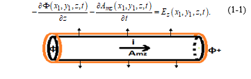Figure I-1 – Segment of the conductor, of length “Dz”, between two scalar potential nodes.

Also, from the equations on the right-hand side of (1) and (3), we have:

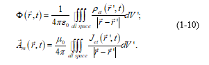
Integrating (1-2) in a closed surface that involves a segment of length “Dz” of the horizontal conductor (see Figure 1-2), we have:

Where: “i” is the total current flowing through the cross-section of the conductor, “I_LS” is the conduction current flowing out of the conductor through the lateral surface, per unit length, and “l” is the free electric charge accumulated on the surface of the conductor, per unit length.

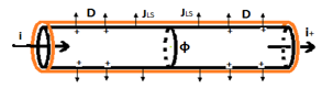Figure I-2 – Segment of a conductor, of length “Dz”, around a scalar potential node.

Equation (1-3) can be interpreted as the application of the Kirchhoff’s law to that particular “potential node”.

If we separate the potentials produced by the matter existing within the segment “Dz” (“A_mz^(Δ)” and “Ф ^(Δ)”), from the potentials produced by the rest of the matter, we have:

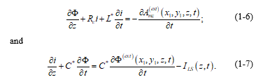
Where: the potentials produced by the rest of the matter,  “A_mz^(ext)” and “Ф ^(ext)”, are the potentials produced by the matter existing in the conductor, outside the segment “Dz”, plus the potentials “A_mz^(ex)” and “Ф ^(ex)” representing the externally applied field; and, “L*” and “C*” are, respectively, the inductance per unit length and the capacitance per unit length of the segment “Dz” of the conductor.

Using Ohm’s law for the conductor, we have:

Where, “R_c” is the resistance, per unit length, of the conductor.

Then, (1-1) and (1-3) can be written as:

As normally, at least a part of the conduction current “I_LS”, flowing out of the conductor through the lateral surface, is due to the linear leakage current, we can write:

Equations (1-6) and (1-9) have the form of transmission-line equations, and, they are completely general and rigorous equations that describe the interaction of an external electromagnetic field with a straight finite segment of a single-wire line, being the only assumptions in deriving these equations: the thin-wire approximation and the validity of Ohm’s law for the conductor.

They can be applied to short horizontal single-wire lines and to long horizontal single-wire lines; also, they can be applied to bent lines, because, in (1-6) and (1-9), “z” represents the direction of the segment of conductor being described, which can be any direction in real space.

Then, they can be applied to different problems, such as, electromagnetic neural stimulation and the calculation of lightning-induced voltages.

As mentioned in reference [1], the main variables in (1-6) and (1-9) are the potentials, which we have seen are very useful for classification purposes. But they are not uniquely determined.

Their values, as well as the value of the inductance and capacitance coefficients, are affected by the choice of the reference point, which is the point where the value of the potentials is equal to zero.

The reference point is normally chosen at the infinity, and with this choice, from (5) we have, in the Lorenz’ gauge, the usual retarded potentials [4]:

Another usual choice assumes the existence of a line along the z direction, where:

This line, which is taken as the reference, could be located at the infinite or very far from the structures of interest, in such a way that the potentials produced by the matter behind the reference are negligible.

Sometimes the reference is chosen on a perfectly conducting conductor. When this perfect conductor has an infinite plane surface, the potentials produced by the matter behind the reference, are represented by the potentials produced by the images of the matter on the perfect conductor plane [13].

       With any choice of reference, as also mentioned in reference [1], Ф in (1-6) and (1-9), can also be interpreted as the potential difference between the conductor and the reference, at a value of z and t.

 In the classical transmission-line theory, which is geared for long horizontal transmission lines, the values utilized, for the capacitance per unit length “C” and for the inductance per unit length “L” of the line, are those calculated, neglecting the retardation effects, for an infinite straight line which is uniformly charged with a charge density, per unit length, equal to “l” and with a current “i” equal in all segments along the line [12]. In this situation, the potentials produced are the so-called static potentials “A_mz^(st)” and “Ф ^(st)”.

We will define the so-called internally-produced potentials “A_mz^(int)” and “Ф ^(int)”, which are the potentials really produced by the matter existing in the conductor; and, we will also define the potentials “A_mz^(c)” and “Ф ^(c)”, which are the difference between the internally-produced potentials and the static potentials.

Writing (1-6) and (1-9) in terms of the quantities defined in (1-12), we have:

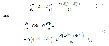To allow an easy comparison with the equations utilized by the people interested in lightning-induced voltages, we will write (1-13) and (1-14) in terms of the internally-produced scalar potential. Then, we have:

To show the generality of (1-15) and (1-16), we will compare (1-17) and (1-18) with reference [13]; where the problem of a single-wire line above a perfectly conducting ground, in presence of an impinging electromagnetic field, is considered.

The result there presented is a system of “generalized” or “full-wave” equations, containing electrodynamics corrections (including radiation) to the standard theory of transmission lines.
Before making the comparison we must note that:

– In reference [13], the total fields are not divided in: internally produced by the single-wire and externally produced, but, they are divided in what they call “scattered fields”, which are produced by both: the single-wire line and its image in the perfectly conducting ground, and what they call “the exciting electric field “E^e”, which is obtained by the sum of the incident field “Eⁱ” and the ground-reflected field “E^r”, both determined in the absence of the wire”.

– Reference [13] only considers an externally impinging electromagnetic field, neglecting the eventual localized external sources conductively connected to the single-wire. Then, the internally-produced potentials reduce to the scattered potentials.

Reference [13] calculates the potentials produced by the matter really existing in the conductor, outside the segment “Dz”, considering the time delay in the production of the potentials. They in fact calculate the potentials “A_mz^(c)” and “Ф^(c)”.

Then, when the perfectly conducting ground is taken as the reference for the potentials, neglecting the conductor resistance, per unit length, “R_c” and the transversal currents “I_LS”, (1-17) and (1-18) reduce to (9) and (10) of reference [13].

2. Comparison of our Field Coupling model with standard coupling theories

Here, as in part 3, we will adopt the same terminology utilized in reference [1].

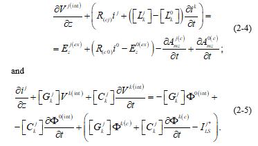
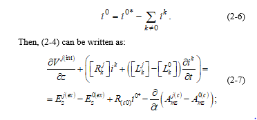
In order to allow an easy comparison with classical transmission-line theories, we will write (34) and (35) in terms of the internally-produced scalar potential. Then, we have:

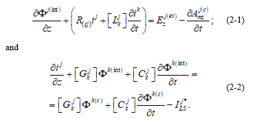Also, in order to compare our results with reference [14], which is considered to represent the classical transmission-line theory [13], for this quasi-longitudinal mode (because of the presence of “I_LS”), neglecting the transversal magnetic potential “A_mt” produced by the transversal current “I_LS”, we will define the internally-produced line voltage with respect to the reference conductor, as in reference [14]:

 The internally-produced line voltage, defined in (2-3), when the external sources conductively connected to the line are not considered, is identical to the so-called scattered line voltage, defined in (7) of reference [14], which is usually adopted in the transmission-line theory utilized by the people interested in lightning-induced voltages [13].

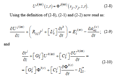
Using the definition of (2-3), (2-1) and (2-2) can be written as:

If we separate, from the current in the reference conductor, the part corresponding to the return current of the other conductors, we can define:

To show the generality of (34) and (35), we will compare (2-7) and (2-5), which are equivalent to (34) and (35), with the corresponding equations of reference [14]:

– Neglecting the differences between the static magnetic potentials and the internally-produced magnetic potentials, the unbalanced current in the reference conductor, and if, from the externally applied electromagnetic field, only the externally impinging or incident electromagnetic field is considered, (2-7) reduce to (16) or (33) of reference [14];

– Neglecting the differences between the static magnetic potentials and the internally-produced magnetic potentials (the electrodynamics corrections (including radiation) mentioned in reference [13]), the non-linear conduction current  I_LS^*, flowing out of the “j” conductor through the lateral surface, and assuming that the internally-produced line voltage is equal to the scattered line voltage, (2-5) almost reduce to (32) of reference [14].

 The terms remaining in the right-hand side of (2-5) come from an assumption that is made here, which is different from the respective assumption made in reference [14]: The capacitance coefficients are here defined in the Maxwell’s way, in terms of the scalar potentials in the conductors; while in reference [14] they are defined in terms of the scattered line voltages with respect to the reference conductor.

Then, as the scattered line voltages represent only differential modes, the remaining terms represent the conversion of common mode into differential mode.

When the internally-produced line voltage “U^j”, in the conductor “j”, is defined with respect to the reference line for the potentials, we have:

Equations (2-9) and (2-10), which are equivalent to (34) and (35), are also completely general and rigorous equations that describe the interaction of an external electromagnetic field with the considered filamentary multi-conductor transmission line, being the only assumptions in deriving these equations: the thin-wire approximation for all the conductors and the validity of Ohm’s law for all the conductors.

Now, if we compare (2-9) and (2-10), with the corresponding equations of reference [14]:
– Neglecting the differences between the static magnetic potentials and the internally produced magnetic potentials (the electrodynamics corrections (including radiation) mentioned in reference [13]), and if, from the externally applied electromagnetic field, only the externally impinging or incident electromagnetic field is considered, (2-9) reduce to (16) or (33) of reference [14];

– Neglecting all the terms of the right-hand side of (2-10) that represent electrodynamics corrections (including radiation) and the non-linear transversal conduction current I_LS^*; and, assuming that the internally-produced line voltage is equal to the scattered line voltage, (2-10) reduce to (32) of reference [14].

Then, we also obtain the advantage for the numerical solution of the system of equations, claimed in reference [14], of having the source term appearing in only one kind of equations.

In fact, this is the formulation utilized for the numerical examples shown in reference [14], which refer to a two-conductor line over a perfectly conducting ground that is taken as a reference plane, not as a reference conductor.

Equations (34) and (35), which are a generalization of (21c) and (22c) of reference [1], as mentioned in reference [1], also represent a generalization of Rusck’s coupling theory [21], by including, besides the corrections due to the time delay in the production of the potentials, the effect of the externally produced magnetic potential along the direction of the line (a shortcoming of that theory pointed out a long time ago [39]) and also the effect of the conductive imperfections of the matter, both of the conductors and of the dielectrics between the conductors.

To include the effect of the transversal mode, we will define the so-called conductor voltages.
Usually, in standard transmission-line theory, the conductor voltages are defined relative to one of the conductors chosen to be the reference [12,30]. Then, to include the effect of the transversal mode, here, we will also define the conductor “j” voltage as the integral of the transversal electric field strength “E_t” between the conductor “j” and the reference conductor:

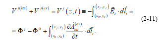Where, as usual, neglecting the transversal magnetic potential produced by the transversal currents, “A_mt” is the externally produced field.

Then, we can modify (34) and (35), by means of (2-11), and obtain:

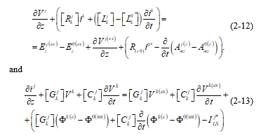In equations (2-12) and (2-13), which are a generalization of (28) and (29) of reference [1], we can also see, as mentioned in reference [1], that writing the equations in terms of the conductor voltages produce new source terms in (2-12) and (2-13), due to the existence of induced voltages produced by the externally applied electromagnetic field.

Apart from the assumptions of the thin-wire approximation and the validity of Ohm’s law for all the conductors, and the assumption that the transversal mode is only externally produced, (2-12) and (2-13) are quite general. Neglecting the terms that appear within the parenthesis in the right-hand side of (2-12) and (2-13), they reduce to (3a) and (3b) of reference [12].

For the special case of time-harmonic electromagnetic fields, or in frequency domain, (2-12) and (2-13) can be written as:

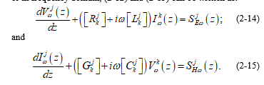Which, without the sources, are the standard transmission-line equations in frequency domain, such as shown in (2) of reference [30] or (6.7) and (6.8) of reference [31].

1.  P. E. Munhoz-Rojas, “Conducted and Radiated Interference on the interconnections of Renewable Energy Farms” in Proceedings of the 2018 Joint IEEE EMC &APEMC, Singapore, 798-804, 2018.
2.  CIGRE Technical Brochure 719, “Power Quality and EMC issues wih future electricity networks”, JWG C4-24/CIRED, www.e-cigre.org, 2018, p.56 .
3.  C. L. Holloway, E.F. Kuester, A.E. Ruehli and G. Antonini, “Partial and internal inductance: Two of Clayton R. Paul’s many passions”, IEEE Trans. on EMC 55(4), 600-613, 2013.
4.  J.D. Jackson, Classical Electrodynamics, 3rd ed., New York: John Wiley & Sons, Inc., 1999.
5.  J.C. Maxwell, “A dynamical theory of the electromagnetic field”, Roy. Soc. Trans. Vol.155, 526-597, 1864.
6.  A. Sommerfeld, Electrodynamics, New York: Academic Press, 1952.
7.  P. E. Munhoz-Rojas, “A Symmetrical Theory of Electromagnetism” in PIERS Proceedings – Moscow2012, 1199-1203, 2012.
8.  R.P. Feynman, R. Leighton and M. Sands, The Feynman Lectures on Physics – The Electromagnetic Field, vol. 2, Reading, Massachusetts: Addison-Wesley, 1965.
9.  Landau, L.D., and E.M. Lifshitz, Course of Theoretical Physics – Vol. 8: Electrodynamics of continuous media, (Spanish translation) Editorial Reverté, Barcelona, 1975, pp. 285-286.
10.  Landau, L.D., and E.M. Lifshitz, Course of Theoretical Physics – Vol. 2: Field Theory, 2nd ed.,(Portuguese translation) Editora Mir, Moscow, 1980, pp. 31, 69.
11.  S.A. Schelkunoff, “Forty years ago: Maxwell’s theory invades engineering – and grows with it”, IEEE Trans. on Education 15(1), 2-14, 1972.
12.  C. R. Paul, “A brief history of work in transmission lines for EMC applications”, IEEE Trans. on EMC 49(2), 237-252, 2007.
13.  F. Rachidi, “A review of field-to-transmission line coupling models with special emphasis to lightning-induced voltages on overhead lines”, IEEE Trans. on EMC 54(4), 898-911, 2012.
14.  A.K. Agrawal, H.J. Price and S.H. Gurbaxani, “Transient response of multiconductor transmission lines excited by a nonuniform electromagnetic field”, IEEE Trans. on EMC 22(2), 119-129, 1980.
15.  P. E. Munhoz-Rojas, “The effect of discontinuities in a multiconductor line on lightning-induced voltages”, IEEE Trans. on EMC 51(1), 53-66, 2009.
16.  A. L. Hodgkin and A. F. Huxley, “A quantitative description of mem-brane current and its application to conduction and excitation in nerve,” J. Physiol., vol. 117, 500-544, 1952.
17.  D. R. McNeal, “Analysis of a model for excitation of myelinated nerve,” IEEE Trans. Biomed. Eng., vol. BME-23, 329-337, 1976.
18.  J. P. Reilly, V. T. Freeman and W. D. Larkin, “Sensory effects of transient electrical stimulation – Evaluation with a neuroelectric model” IEEE Trans. Biomed. Eng., vol. BME-32, 1001-1011, 1985.
19.  F. Rattay, “Analysis of models for external stimulation of axons” IEEE Trans. Biomed. Eng., vol. BME-33, 974-977, 1986.
20.  B. J. Roth and P. J. Basser, “A model of the stimulation of a nerve fiber by electromagnetic induction” IEEE Trans. Biomed. Eng., vol. BME-37, 588-597, 1990.
21.  S. Rusck, “Induced lightning overvoltages on power transmission lines with special reference to the overvoltage protection of low voltage networks”, in Trans. of the Royal Institute of Technology, Stockholm, Sweden, vol.120, 1958.
22.  T.W. Dawson, J. de Moerloose and M.A. Stuchly, “Hybrid finite-difference method for high-resolution modelling of low-frequency electric induction in humans”, J. of Comp. Phys. 136, 640-653, 1997.
23.  X.L. Chen, S. Benkler, C.H. Li, N. Chavannes and N. Kuster, “Low frequency electromagnetic field exposure study with posable human body model” in 2010 IEEE International Symposium on Electromagnetic Compatibility, Fort Lauderdale, FL, USA, 702-705, 2010.
24.  P. E. Munhoz-Rojas, C.S. Segura-Salas, A.A. Costa, R. Martins and J. Hoffmann, “Fields and current densities induced in the human body by low-frequency electromagnetic fields” in Proceedings of the 2018 Joint IEEE EMC &APEMC, Singapore, 1267-1273, 2018.
25.  J.C.Maxwell, A Treatise on Electricity and Magnetism, 2nd Edition, Vol. II, Oxford: Clarendon Press, 1881, pp.207-208.
26.  J.C.Maxwell, A Treatise on Electricity and Magnetism, Vol. I, Oxford: Clarendon Press, 1873, pp.89-90.
27.  L. F. Shampine, Numerical Solution of Ordinary Differential Equations. New York: Chapman & Hall, 1994.
28.  C. R. Paul and J. W. McKnight, “Prediction of crosstalk involving twisted pairs of wires-Part I: A Transmission-line model for twisted-wire pairs”, IEEE Trans. on EMC 21(2), 92-105, 1979.
29.  G. Spadacini, F. Grassi, F. Marliani and S. A. Pignari, “Transmission-line model for field-to-wire coupling in bundles of twisted-wire pairs above ground”, IEEE Trans. on EMC 56(6), 1682-1690, 2014.
30.  S. Greedy, C. Smartt, M, Basford and D. Thomas, “Open source cable models for EMI simulations”, IEEE EMC Magazine 7(3), 69-81, 2018.
31.  CIGRE Technical Brochure 707, “EMC in wind energy systems”, WG C4-30, www.e-cigre.org, 2017, pp.45-46 .
32.  C. A. Nucci, F. Rachidi, M. V. Ianoz and C. Mazzetti, “Lightning-induced voltages on overhead lines”, IEEE Trans. on EMC 35(1), 75-86, 1993.
33.  A. Tatematsu, F. Rachidi and M. Rubinstein, “A technique for calculating voltages induced on twisted-wire pairs using the FDTD method”, IEEE Trans. on EMC 59(1), 301-304, 2017.
34.  P. Munhoz-Rojas and C. L. da S. Pinto, “Analysis of lightning-induced voltages on an overhead line” in Proc. of. 8th Int. Symp. Lightning Protection, Sao Paulo, Brazil, 57–62, 2005.
35.  S. Yokoyama, “Calculation of lightning-induced voltages on overhead multiconductor system”, IEEE Trans. Power App. Syst., vol. PAS-103, no. 1, pp. 100–108, Jan. 1984.
36. M. Paolone, C. A. Nucci, E. Petrache, and F. Rachidi, “Mitigation of lightning-induced overvoltages in medium voltage distribution lines by means of periodical grounding of shielding wires and of surge arresters: Modeling and experimental validation”, IEEE Trans. Power Del., 19(1), 423–431, 2004.
37.  P. E. Munhoz-Rojas and C.L.da S, Pinto, “Calculations of lightning-induced voltages in distribution lines with LSA”, Journal of Energy, 60, Special Issue, 95-100, 2011.
38.  Hertz H., “The forces of electric oscillations, treated according to Maxwell’s theory” (in German), Wiedemann’s Annalen, 36, p.1, 1889. (English translation in Electric Waves, by Heinrich Hertz, translated by D.E. Jones, MacMillan and Co., London and New York, IX,137-159, 1893).
39.  V. Cooray, “Calculating lightning-induced overvoltages in power lines: A comparison of two coupling models”, IEEE Trans. on EMC 36(3), 179-182, 1994.

(Click Here)

(Click Here)