1. Notification of Intent

This paper is an extension of work originally presented at the 2017 National Aerospace & Electronics Conference (NAECON) [1]. In this work we illustrate the ability to utilize formal methods and automated theorem proving (ATP) to discover errors in specification development prior to implementation. A major concern addressed from feedback at NEACON 2017 is the prevention of errors in the proof environment. We expand on that work by showing that formal methods and ATPs can be used to find errors in the proof of function correctness. This allows for a system of checks and balances between specification and proof development for formal methods, verifying that both parts adhere to the original customer requirements.

This paper also extends work originally presented in 2016 at the Midwest Symposium on Circuits and Systems (MWSCAS) [2]. In that paper we addressed the use of statistical metrics to show the reliability of software over time. This process relies on the use of techniques we developed to define independent, random errors for injection into our elevator controller benchmark program. However, our presentation of those techniques was brief due to page limitations and the need to discuss the results of our testing procedure for software. To address the feedback on that work, we will be elaborating in depth on our technique for generating random, independent errors using real-world reported error results and random number generators (RNGs). This also includes a discussion of how we determine the best RNG for our needs.

Finally, this paper extends work originally presented in 2018 at MWSCAS [3]. This was originally an expansion of our work in [2] using a different error rate and looking at possible better statistical models of reliability for software. Many of the commentators on our work suggested expanding the results to more programs and improving the results by looking into focusing the data, as some outliers had caused degradation in the results. We address both of these points by expanding the testing and analysis to five more programs, using characteristics and style similar to our original elevator controller benchmark, and then developing a process to remove outliers in the data through the use of statistical measures.

2. Introduction

Embedded systems in recent years have taken a leap in their integration with everyday society. They appear in various forms from wearables, to cellphones, to the vehicles we drive; it is important that these embedded systems function correctly. In many fields, such as medicine and aerospace, there is a strong focus on these systems being secure, reliable, and robust. These trusted and safety critical systems must work correctly as their failure could result in injury or, in the worst case, the loss of life of those that are dependent on them.

Many trusted systems encountered today utilize hardware specific embedded systems. Hardware has a tradition of reliability and safety, because of its use of industrial practices and standards. In VLSI design, developers can compare their working designs to standardized benchmarks (e.g., MCNC [4], IWLS [5], and LEKO [6]) and this generates a baseline of confidence in the design. Beyond benchmarks, tool designers have incorporated Model Checking [7] into their development suites, allowing for reliability checking against industry determined “golden models” [8–11]. These techniques are invaluable in generating the statistical models of reliability for hardware systems.

Unfortunately, the constraints of Moore’s Law [12,13] and the increased complexity of system function have required a change in the design approach of critical embedded systems. Some industry practice has attempted to maximize the resources available for a given space [14–17], but these techniques are fairly new, and VLSI tools and techniques are lagging behind in allowing for these techniques, slowing adoption. Other researchers are looking at maximizing the capabilities of current hardware by focusing on implementing machine learning in embedded systems [18]. However, this is difficult to achieve for safety critical systems with the large overhead that comes with high precision computing with machine learning [19].

Hence, software is an attractive alternative for meeting the demand for complex, real-time critical systems. Several recent disasters (e.g. [20–22]) have, however, indicated that the current process of testing to exhaustion and representing software reliability as defects per thousand lines of code (ELOC) [23] is not sufficient. This is especially true when taking into account the fact that there is no industrial standard for counting “lines of code” and factors such as size play a role in misrepresenting results [24]. Software metrics similar to hardware would be ideal, and theoretical work in this area has shown software should be able to be modeled with statistics [25–30]. Government agencies have also released standards of development [31,32] to provide a framework for illustrating reliability effectively. However, there is no specific development process outlined for achieving either of these improvements.

The work presented here is a complete development process that we propose for use in addressing the challenges described above. This development process allows for the establishment of a suite of benchmark programs, defining a baseline similar to hardware which other trusted systems utilizing software can be compared to. This suite is open ended and allows for the addition of more programs in the future. To accomplish this goal, we will address the area of specification design through the use of formal methods, and show how errors can be eliminated early in development with the use of ATP. This work is an expansion of work already presented in [1,33]. We will also illustrate the development, use, and statistical results for reliable software in safety critical applications. This approach has been briefly presented previously in [2] and improved in [3]. We expand upon those findings to complete the suite of small embedded programs which establishes the initial set of well-defined benchmarks for software reliability and a baseline for software testing.

3. Related Work

There have been several groups researching the use of formal methods in the recent literature. This work has targeted two main areas. The first is the use of model checking with software, and the second is the improvement of ATPs. One area of use for model checking is for reverse engineering a system [34]. Since automated implementation is not available yet for specifications written in formal methods, the reverse engineering process uses the implementation to move back to a specification, verifying it is correct with model checking, and then verifying the original specification and reverse engineering specification are correct with respect to each other. Another area is related to the development of a tool called Evidential Tool Bus (ETB) that combines both model checking and ATPs into a single environment to allow better verification of specifications written in formal methods [35]. Finally, researchers are looking at the inclusion of model checking into development tools to use in verifying that object oriented programs are correctly implemented [36]. This process is similar to the current tools for model checking hardware designs provided by Synopsys [7].

The research in improving ATPs has involved making them more inclusive for developers. Currently systems such as ProofPower [37], although powerful, require the user to know the formal method and ATP language for proof verification. Some work has been done to provide a more mathematical environment to work in, replacing the intermediate ATP language, i.e SML, with mathematical notation. Some of this work includes the use of superposition calculus [38], modal logic [39], and standard calculus [40]. Other researchers have looked at changing the language of formal methods and ATPs together, working to use traditional programming languages from the beginning of specification design, and this work has focused primarily on the language LISP [41]. These changes would require a change in the current specification writing practices with formal methods [42,43].

Current work in the field of software development has focused on improving the metrics of throughput and performance for large scale, big data [44] applications. This work includes generating heuristics for quality assurance (QA) [45] with probabilistic analysis, and attempting to predict where in the development life cycle a particular project will have the most errors [46, 47]. This allows developers to focus their efforts in those areas to mitigate the time and cost for a given project. Machine learning is assisting in this field, where it is used to predict the optimal release time of a given system based on the metrics of testing, cost, and errors produced [48]. Many of these techniques are being applied specifically to projects that rely on cloud computing [48] and open source software [49]. They are not being used to directly target the component level reliability which is required for safety critical systems and those relying on software in an embedded environment.

4. Background Knowledge

Formal methods are supported by many languages, such as Z [50] and VDM [51], that share in common a reliance on basic mathematical principles. These principles include axiomatic notation [52, 53], predicate calculus [54,55], and set theory [56,57]. When combined with the formal methods syntax, these principles allow us to develop specifications describing the functionality of a system [22,58]. These principles are often taught in engineering course work, and formal methods often have manuals describing how the language operates [59], similar to a conventional programming language such as C or Java.

One important aspect, however, is the mechanisms through which formal methods have traditionally been used to show that a given method in a specification is correct. The traditional method is to prove a specification is correct through a process of refinement. This process requires “refining” a particular part of a specification written in formal methods to an implementation method, such as analog circuitry or Java, for a particular portion of the specification. This decision to refine to a particular implementation is required ahead of time so there is a goal to achieve for the refinement. Later changes to the implementation require that a new proof via refinement be performed. Understanding this process and why our work has moved in a more modern direction is important and we illustrate this process in the following example.

The example we are working with will utilize an elevator controller benchmark as originally described in [33] and referenced in Section 5. The elevator controller discussed here has requirements presented in Figure 8. For the refinement process, we will use Z for the formal specification language and C as the implementation target. Note that any formal method and implementation medium can be utilized for refinement as long as the characteristics of each are well understood and the proof can be completed. In contrast to the original requirements of [33], some additional constraints need to be in place before the refinement can proceed. In particular, the constraints are:

• The model will illustrate the action of users in the system; specifically we will model the entry of passengers onto the elevator
• People are unique individuals
• Entry into the elevator is sequential
• The elevator can move with or without people
• There is no max capacity
• The system contains one elevator

With these extra constraints on the system defined, the refinement proof can begin. The first step is to develop a definition of the possible group of users for the elevator. Since we used the wording in the constraints, we shall refer to these users as “People.” We use Z to define “People” as a “Set,” because sets are flexible and convenient for developer definitions in Z. Figure 1 illustrates the definition of “People” in Z.

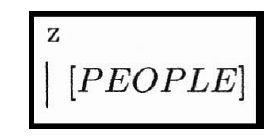Figure 1: Z definition of the set “People”

Now that the generic definition of “People” has been established, we need to define a subset of “People” who will be using the elevator. To ensure that the specification is as open as possible we will define the subset of “People” who are riding the elevator via a power set. This way any combination of members of “People” can become “riders.” Figure 2 captures the creation of this power set using the Z construct known as a state in ProofPower [59].

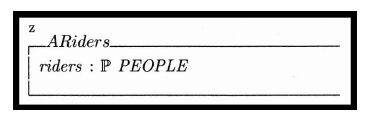Figure 2: Generic state sefinition for the power set “Riders”

The final part of the initial definition is to describe the act of getting on the elevator. In Z this can be done using a function declaration, which will include a change in the state of the system and a member of the set “People” becoming a member of the power set “riders.” Figure 3 shows the generic definition for this function.

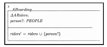Figure 3: The generic function definition for boarding the elevator

Now we need to complete the same process but with the implementation medium we have decided on. As mentioned, we have chosen C for this task. The first step is to define the state of the system as it would be represented in C. We will reuse the same set “People” we defined previously for this task. In a programming language such as C, sets of items are usually stored in an array or a linked list. This is what we would use to store the members of the set “People” who board the elevator. However, Z does not have these constructs directly, though it does have a structure that an array or linked list can be modeled in, and that is a sequence. A sequence is a good comparison as a set is equal to the range of a sequence, as shown in (1).

In this equation s represents the set, ran is the notation for range, and ss represents a sequence. Now we construct the state of the system with Z for C using the sequence term seq, and generating a new, more specific group called “riderss.” Figure 4 shows the construction of this state.

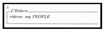Figure 4: State for “Riderss” in C using Z

Finally, we complete this portion by describing the action of a new rider boarding the elevator in C. Since we are dealing with a sequence, the mathematical notation we will use is a concatenation. Figure 5 shows the state for C as defined in Z.

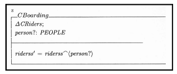Figure 5: C function definition for boarding the elevator

With the set “People” we have now defined two versions of the system for boarding the elevator, a generic one which describes the basic functionality and a more specific one constrained by the properties of our implementation medium C. This gives us a starting and ending place. To bridge the gap between the two and what they describe, we need to develop a proof to show that the generic function can become the specific function. To start we build a proof implication, or goal, illustrating this transformation. This will be done using Equation 1 for some replacements for riders and riders’ from the generic definition in Figure 3. Figure 6 gives the initial implication, showing the end requirement for the C definition from Figure 4 and using the previous set to sequence rule to rewrite riders and riders’ in terms of the range for riderss and riderss’, respectively.

To complete the proof implication, we want to drive one side or the other to an absolute true which means everything on the other side must hold as defined. Since the outcome only has one statement, this is the easier of the sides to work on. Figure 7 shows the seven step proof indicating the implication holds and the refinement is true.

Using set theory and rewrites of variables taken from the specifications, we are able to show that the generic specification can be refined to the specification for C. This was a simple example and even then it took seven steps to complete, along with a strong knowledge of the constructs of Z, C, and set theory. To attempt to complete a definition for a more complex system and multiple functions would be very time consuming and may cost more than just using traditional testing methods due to the time involved. Furthermore, this process does not define the function in a useful manner that would assist with the conversion to an implementation, but rather shows the theoretical correctness of the system definitions for a particular implementation medium. Even when using an ATP to perform the refinement steps, the final implementation may not be correct in a functional sense, as the definitions are mathematical, not practical. Hence our work [1,33] described in Section 5 and extended in Section 6 shows the advantages of utilizing a functional specification and proving that correct. It also provides the flexibility of being implementation neutral so a new proof does not need to be constructed if the implementation medium changes.

Figure 6: Implication definition for showing the refinement steps

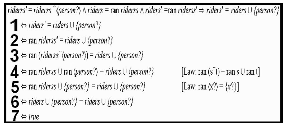Figure 7: Proof showing the refinement of the specifications using Z

One final area of background work that we utilize for our error analysis is the theory that software errors can be modeled as a Non-Homogeneous Poisson Process (NHPP). A NHPP is defined well in the sources [60–63]. The important factor for our work is that software errors were shown to meet the requirements of a NHPP in [29], which originally had been theorized in [25, 26, 30], and shown to fit statistical models in [28]. The takeaway is that software errors have been shown to fit NHPP, implying that these errors occur at random intervals and that they are independent of one another. This allows us to define our error generation and testing procedure, discussed in Sections 7 and 8 and in the results presented in [2,3].

5. Specification Development with Formal Methods

As shown in Section 4, an understanding of refinement is important for developing specifications and proofs for showing the system design is correct. However, this traditional methodology limits the scope of the system to a particular implementation method. The implementation chosen for the proof reduction my not be the best for a given system process later in development. If a new implementation is chosen, then a new proof will need to be created to drive the specification to that implementation, resulting in the development of new state diagrams and another refinement. This correction in the design would be costly in the time required for the refinement.

In previous work [33], we utilized a simple elevator controller, in the style of Moore and Mealy Machines, to show that an implementation independent specification could be developed and proven correct without the need for traditional refinement. This was done using “Z” [50] and the Automated Theorem Prover (ATP) “ProofPower” [37]. Figure 8 shows an excerpt from [33] with the initial customer requirements for the simple elevator controller.

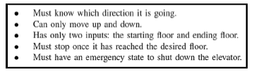Figure 8: Customer requirements for our elevator controller

From these requirements we are able to build a complete specification and proof illustrating our formal methods design process [33]. This added step in development does add time to the process, just like refinement, but there are strong benefits to its use over refinement. This includes focusing the functionality of the system, making it less likely errors will occur during the implementation step [33], since the specification is designed in a similar style to function definitions in software. This also eases the transition when building an implementation from customer requirements. Another benefit is finding development errors prior to implementation [1], which is usually a cost saving measure compared to finding errors later in development. There is also the added advantage of not having to refine the specification to a particular implementation, while maintaining the advantage of proving the system correct.

The error now is in the proof goal set by the independent tester, causing the goal statement to be calling f loor? ≥ starting f loor?, which is shown in Figure 10.

6. Using Formal Methods to Eliminate Design Errors

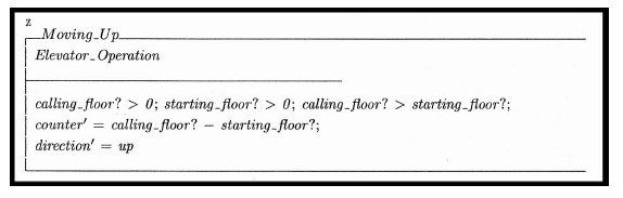Figure 9: “Moving Up” function represented in Z

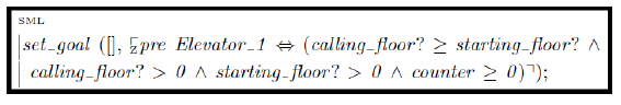Figure 10: Proof goal for “Moving Up” with an incorrect math statement

An important advantage to using Formal Methods is to allow for design flaws to be determined prior to the system reaching implementation. Often a customer’s requirements may have conflicting or impractical goals which cannot be determined until they are built into the system. Formal Methods proves those requirements are sound prior to implementation, decreasing the time of development and the cost to remove errors later in development. However, human error can still plague the development life cycle.

Human error in development can come in many forms, but one such error in software design comes from the developer accidentally injecting an error into the system. For example, misspelling a variable name so it matches a similar variable could cause a drastic change in the functionality of the system. Another example is changing an addition to a subtraction, which could be accomplished with an errant key stroke. To combat these errors, independent verification is used in testing, helping to eliminate the bias a developer may put unknowingly into their own tests. This concept works equally well with Formal Methods.

In our work [1] we previously showed that independent verification during the proof of a specification enabled errors to be found and eliminated prior to implementation. Feedback on this process noted that the error could be propagated from the specification to the proof, causing it not to be caught. We emphasize that specification and proof development should be completed by separate individuals, allowing for independent verification. It is unlikely that two developers would make the same mistake by misinterpreting the customer requirements. This does however bring up a separate issue, i.e, that the mistake could be with the proof and not with the specification. Would the proof environment be able to locate an error in the proof statement, given a correct specification? This is the question that was posed, and this is what we have set out to determine.

In [1] we utilized the “Moving Up” function as test and that is the function utilized here for consistency. Our work in [1] showed that a slight change in the specification over the customer requirements could cause a dramatic change in how the system functioned. In this case the original requirements, as shown in Figure 8, require that, if the elevator moves up, the floor it is going to has to be a higher value than the floor the elevator starts on. This is represented in the specification as calling f loor? ≥ starting f loor?, where ≥ has replaced the correct term >.

Now, consider the reverse situation. The original requirements have remained the same from Figure 8, and now the specification for “Moving Up” is correct as it is in [33], shown in Figure 9.

With this mistake in the proof, the proof begins with a goal that is less strict than the specification, in that “greater than or equal to” is more inclusive than “greater than.” Much like our previous use of ProofPower in [1, 33], we need to drive the proof to completion, attempting to resolve all goals defined in Figure 10 via a series of commands issued to the ATP. Figure 11 shows the current steps we will use to try to prove the specification is correct.

Step 10 in Figure 11 is where the proof fails. Figure 12 shows the output from ProofPower when the exception is thrown and the proof can not be completed. ProofPower is reporting that the original goal as stated can not be proven given the assumptions and constraints on the proof, which were set in the original specification.

Unlike the original error recognition test in [1], the semantics error takes longer to find when the error is in the proof goal; nevertheless the error was found, even when it was within the proof goal definition and was weaker than the original specification. Overall, the exception shows that there is an issue with the system, either with the specification or the proof. At this point it would be up to the proof writer and the developer to review their respective sections with regards to the customer requirements and to determine where the error occurred.

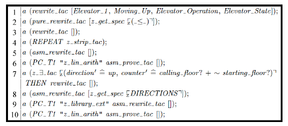Figure 11: The steps necessary to complete the proof to show the goal is correct

Table 1: PSP program line count and error results Language Program Total Lines of Code Total New Lines of Code Number of Errors C++ 1 82 82 12 2 233 233 31 3 463 263 24 4 236 129 15 5 178 104 19 6 568 299 40 7 678 86 20 8 458 298 47 9 824 258 35 10 1202 379 62 TOTAL 4922 2131 305 Eiffel 1 70 N/A 6 2 82 N/A 17 3 214 N/A 19 4 220 N/A 8 5 182 N/A 13 6 396 N/A 28 7 286 N/A 11 8 444 N/A 20 9 784 N/A 23 10 766 N/A 36 TOTAL 3444 N/A 181

Finding errors early in development, as in this example or previously in [1], is invaluable to the development process. This allows you to find semantic errors that are caused by developer mistakes prior to those errors being propagated into the implementation. If this were to occur, there is no guarantee that the error would be caught in the testing phase, and thus it could require a change to the system after release, costing extra time and money. Finding errors earlier in the development process is usually more cost effective, and utilizing a well developed ATP like ProofPower should help eliminate development errors prior to implementation.

7. Developing Repeatable Errors from Real World PSP Results

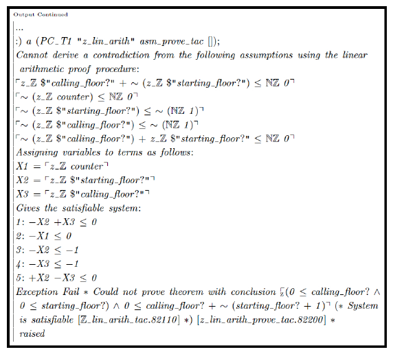Figure 12: “ProofPower” output from failing step ten in the reduction process

Before moving into implementation and testing, it is crucial to have repeatable results. In our case, this means not repeatedly injecting the exact same system errors. This is important as the premise of some of our work goes back to the work done by Yamada [29,64], as explained in Section 4. Our errors need to be random and independent of one another for them to fit into the model of an NHPP. This will not be the case if the same errors are used for every evaluation of our procedure. To that end we turned to the work of Victor Putz [65] who created examples using PSP [66] to illustrate its ability to assist a developer in becoming more proficient in software development. Through the posted results we are able to catalog the findings, developing metrics to allow us to generate error rates and determine errors for replication in our test system. Putz performed a self-exploratory study through PSP, publishing the information for each step in the training process, along with the code he developed, his thoughts, issues, experience, and results [67]. He used a chart system to categorize each error that he made for each program, and an example of this report can be found in [68].

There are altogether ten programs developed through the PSP training, and many of the previous programs build on one another. In Putz’s analysis of the training, he went through the process using two different languages, C++ and Eiffel. Each language had its own unique set of code [67], and statistics for each based on the program developed. C++ did have better reporting as compared to Eiffel, but regardless, based on the information and programs reported for each chapter, we were able to collect data from the study. Table 1 shows the results we collected from what was presented by Putz.

Between the two programs, C++ had total lines developed and total new lines added (for programs that were expanded upon), whereas Eiffel just had the lines for each program developed. Despite this we are able to determine several error rates, two from C++ and one from Eiffel. Eiffel’s error rate was calculated by taking the total number of errors committed and dividing it by the number of developed lines. This rate is 5.26%. C++ programs yielded two error rates, one from total developed lines and one from total new lines added, with both being divided into the total number of errors committed in the ten programs. This gives us two very different rates for C++, with one being below ten errors per lines of code (ELOC) and one over. The high error rate for C++ is 14.31% and the low error rate is 6.2%.

Now that we have rates to use to inject errors into a system per one hundred lines of code, we next need to establish what error groups were reported. From the result tables, like the one in [68], we can see that each error is coded, and a text description of the error and/or its resolution is provided. We refer to the chart Putz posted on his site to get the categories and their meaning [69]. Using this information we are able to generate a list of the errors that appeared during his independent study of PSP. From the error categories and definitions, along with examining the code, we were able to break the errors into groups. We then determined the errors made for each type in each program for C and Eiffel. Table 2 lists the errors of each of the types for each program along with their totals.

Based on the categories of errors presented, we determined what errors could and could not be replicated using automation. The errors categorized as “Algorithm Alteration,” “Missing Algorithm,” “Specification Error,” or “Unknown” are more overarching, sometimes requiring a redesign of a whole algorithm, and would be too difficult to reproduce automatically. Those errors should occur anyway in the implementation and testing process for a developer, so our programs should have representatives of these errors included in them naturally. The remaining errors could be replicated via selection, which is addressed in Section 8, because they affect a specific point in the code, requiring up to only a few changes to correct. Table 3 shows the final selection of errors chosen for replication along with the rate at which they occur during the PSP process. These rates were calculated by taking the total found for a specific error and dividing it by the total number of errors for error types we can replicate.

Table 2: Total erors made by type for C++ and Eiffel

Error Type	C++	Eiffel	Total
Spelling	29	26	55
Used Wring Type	52	26	78
Missing Header Information	21	6	27
Incorrect Math Operation	28	33	61
Incorrect String Operation	11	10	21
Error Handling	13	2	15
Passing Parameters	12	3	15
Conditional Error	10	11	21
Incorrect Method	16	16	32
Missing Block/End Line Character	30	12	42
Algorithm Alteration	31	18	49
Missing Algorithm	37	15	52
Specification Error	11	2	13
Unknown	4	1	5

Table 3: Percentage of Errors Made by Type

ErrorType	Percentage
Spelling	14.99
Used Wrong Type	21.25
Missing Header Information	7.36
Incorrect Math Operation	16.62
Incorrect String Operation	5.72
Error Handling	4.09
Passing Parameters	4.09
Conditional Error	5.72
Incorrect Method	8.72
Missing Block/End Line Character	11.44

From the diagnosis of Putz’s results we have been able to develop error rates to use for injecting errors into our system, and rates for error types that we can replicate. This will be valuable and completes the first step, namely the need for independent errors. The next step will be formulating a way to determine which errors will occur, how many will occur, and where each will be injected into the system.

8. Generating Random Errors for Insertion Into a System

Previously in [2] we briefly discussed an analysis to determine a good RNG for use in replicating random errors. A critique from the results presented was the need to test the RNGs at all. The most critical response to this is that the errors being generated need to be random and independent of one another such that the errors will fit the aforementioned NHPP. Unfortunately, RNGs for general computing, such as rand() that comes with C/C++, are only pseudo-random. This means that there is a pattern to the numbers being generated and it could be predicted. If the values are predictable then the numbers generated are not random and therefore will not fit NHPP.

Tests have been generated over the years to determine the randomness of an RNG, e.g., by Knuth [70,71] and Marsaglia [72]. However, these tests are singular and require the tester to input parameters to constrain the test. This allows an RNG developer to design their generator to defeat one or two of the tests chosen to show randomness. Fortunately L’Ecuyer has provided a solution to this issue with the TestU01 package [73]. This C package combines multiple tests from multiple authors, and has been calibrated in such a way that each test is given the correct parameters for the level of testing being performed [74]. For this work we will be utilizing the test suite L’Ecuyer calls SmallCrush as it is described as sufficient for determining if an RNG is suitable for general computation [73]. All inputs and test generations for TestU01 have been determined by L’Ecuyer using statistical analysis [74], and in the case of SmallCrush the total number of values generated for each test is approximately 5 million values, which we validated through testing.

Using SmallCrush we can determine an RNG that can be considered sufficiently random and allow for meeting the requirements for NHPP. Rand() was decided upon as a baseline for utilizing SmallCrush and generating results to see what tests it would pass. Rand() was also chosen as the baseline since it is the default RNG included with the C/C++ library. Testing with SmallCrush was completed three times for consistency, on integer and decimal values, and was initially seeded at the start of each test with the current time to prevent starting at the same value for each test. Figure 13 shows the an example of the output from SmallCrush using rand() to generate integer values, and Figure 14 shows the final results for rand() generating integer values.

The results show that rand() for C/C++ fails twelve of the total fifteen tests (passing only three). This is consistent for the next two runs, failing the same twelve tests each time. Now with this baseline we can move on to see if we can find a better RNG, needing one that can pass all fifteen tests to be considered “random.”

We want to minimize the development of tools and inclusion of extra libraries, so finding a generator that can be random for both integer and decimal values is optimal. Researching the literature, one in particular that appears to meet these requirements is PCG32 by O’Neal [75]. This RNG has a small extended footprint with its included libraries, and the results show that PCG32 has already passed SmallCrush. We will independently re-evaluate these claims. Other RNG designs were considered, such as SBoNG [76], but they have already been shown not to be “random” [77] via SmallCrush.

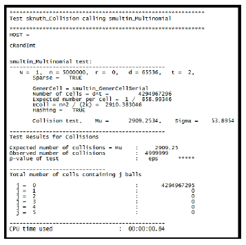Figure 13: Output from SmallCrush testing rand() RNG

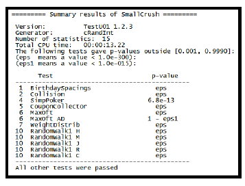Figure 14: Final results for rand() when tested with SmallCrush

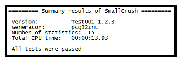Figure 15: Final results for PCG32 when tested with SmallCrush

PCG32 was tested three times each for consistency, just like previously with rand(). Figure 15 shows the results for one run of PCG32 generating integer values. All three runs through SmallCrush resulted in the same outcome.

The results from this testing are impressive. The results show that PCG32 performs as claimed [75], passing each of the tests for all three runs. It has proven to be sufficiently random for general computation and allows us to generate the random values necessary for compliance with NHPP.

9. Random Error Generation

Before we can evaluate our testing procedure, we need to generate random errors for the system using the error rates we determined in Section 7. This is subdivided into three parts:

1. Count the lines of code for each benchmark program in a consistent manner
2. Determine the possible injection points for each error we will replicate; this will need to be done for each benchmark program
3. Randomly select the number of errors to occur, which errors will occur, and where in the program using the derived data from the PSP analysis

Item 1 is the first to be addressed. An automated method for determining the number of lines for each program is critical for the count to be consistent and accurate for each benchmark program. Unfortunately there is no industry standard for counting lines. Many reports have proprietary methods of counting lines, such as compiled compared to written, or counting spaces versus not counting spaces. This is typically used to help improve the error rate for ELOC representation, as mentioned earlier. In our case, in reviewing the lines reported by Putz, and reviewing our own benchmark programs, it was determined that the fairest and most consistent measure would be to count the lines of written code that would be compiled. This means only complete lines would be looked at, and unnecessary spaces and trialing lines with braces would need to be eliminated. This would compress the written code down into lines to be compiled while allowing each required statement to be on its own line. Figure 16 shows an excerpt of code from our elevator controller benchmark after it has been compressed by the line counter.

The results show the extent of the function of our counter, removing unnecessary space for the functions of the code (usually they are for clarification), and comments (which are not necessary for function and skipped by the compiler). Also, braces have been moved to the last complete line that requires them (meaning that some lines have multiple braces from nesting). Overall, this makes for a compact and fair result. Each of our six benchmark programs was processed through the counter. Table 4 shows the final lines counted for each program.

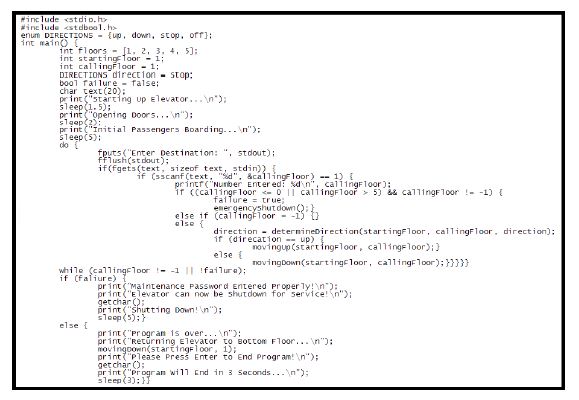Figure 16: Elevator controller code after being parsed by our line counter

Table 4: The line counter results

Program	Total Lines Counter
Elevator Controller	96
Automatic Door Controller	62
Security System	89
Streetlight	83
Tollbooth	54
Vending Machine	61

The next step is Item 2. This proved difficult to automate, as the C library is vast, and developing a parser to incorporate all the possible injection sites for each of the error types could not be completed. In the future we plan to automate this process, but for now this was completed by hand through scanning the code for each error type and marking an injection site with a value, and then counting the number of places an error could be injected. Some errors had overlap, so care will need to be taken to incorporate both errors if there is overlap when injection sites are randomly selected.

Finally, Item 3 is completed. Our program allows us to input the number of lines determined from the line counter program, and the number of places each error can be injected. The error selector is hard coded with the C++ high and low error rates determined in Section 7, as those will not change. The algorithm uses the rate, which is a percentage, the average errors seen per one hundred lines of code, and then determines the number of errors that should be injected into the current program. For example, if the program had two hundred lines of code, then, based on the high error rate, 28.62 errors should be injected into this program. Since we can not generate fractional errors, the system rounds up to the nearest integer for rates x.y where .y ≥ .5 and rounds down to the nearest integer for rates x.y where .y < .5. In a similar fashion, using the total number of injected errors just calculated, the program calculates the number of errors of each type to generate. This is done by having PCG32 generate a decimal value z within the range 0 ≤ z ≤ 100. The previous error percentages are now on a scale from 0 to 100, with subdivisions ending with their rate plus the previous rate. Table 5 shows the range for each error.

Table 5: Repeatable error ranges for random generation

Error Type	Decimal Range

The system repeats the process of using PCG32 to generate a value and comparing it to the scale in Table 5 until all errors for the system have been generated. Table 6 shows an example of the number of errors of each type selected randomly for a single run of the program for the Elevator Controller for the high error rate.

Finally, the last step is to determine the locations for the errors to be placed for the number of each error selected. These locations are also randomly selected using PCG32. For example, Table 6 shows that, for the Elevator Controller, 3 spelling errors are to be made. Using the selected number of errors by type, and the total number of places in the code that error can occur, the system randomly selects the locations for injection into the elevator code. The system is configured not to select the same injection site more than once.

Table 6: Error selection for the first elevator test run

ErrorType	TotalGenerated
Spelling	3
Used Wrong Type	2
Missing Header Info	1
Incorrect Math Operation	1
Incorrect String Operation	1
Error Handling	1
Passing Parameters	0
Conditional Error	2
Incorrect Method	0
Missing Block/End of Line Characters	3

For multiple testing runs, the program is run multiple times to generate a unique set of error injections for each run of a program, with no two runs being alike. For our testing, each program is going to be put through the testing procedure ten times, which requires ten selections of error types and locations to be processed. This process is then repeated for the low error rate as well, giving us a combined twenty unique error profiles for our program. Therefore, with this process, no program will have the same errors from testing iteration to testing iteration, allowing for a random error removal process as errors are discovered.

10. Data Collection Using Elevator Controller

Previously in [2] we illustrated a four state testing procedure. To re-cap, this process occurs as follows: (i) Compilation, (ii) Static Analysis, (iii) Compilation After Static Analysis (CASA), and (iv) Testing. From each of these stages, errors are determined and removed, and the time taken to locate all errors is recorded for each stage. Each stage’s time and error count is combined, respectively, giving us total errors found during a testing iteration. Testing iterations are repeated until no more errors are located in all four stages.

A database is utilized to store the errors found. We built our database in Microsoft Access as it comes configured to allow the use of style sheets for inputting data entries, and it was easy to build a single repository to include all runs for each error rate for each program. By incorporating slots for time, location in the code, and the categorization method from Putz [69], we have created a comprehensive form that shows the discovery and removal of each error in the system being tested. Figure 17 shows the entry form for the database, and Figure 18 shows an excerpt from the table of entries after errors have been entered.

This digital recording method is faster than trying to record errors by hand and allows the developer to focus on finding and removing errors in a timely manner. This helps to reduce bias in the data and exclude as much as possible extra time that might be taken up by writing the findings down or using other recording methods. This also allows the developer to have a digital repository of their error findings, allowing them to see possible improvement from program to program as they utilize our testing procedure.

11. Results and Data Analysis

Using the testing procedure described in Section 10 and explained in [2], we completed ten runs for each error rate on our starting example the elevator controller. The results [2,3] showed that using our complete development process, from formal specification through testing, demonstrates that software systems can use error metrics that fit statistical models, as originally proposed by Musa [25, 26] and Drake [30]. Further refined models [29] were explored in [3] but were inconclusive as to whether they were better than the base exponential model. This required further testing.

Now we have completed the same testing procedure on our remaining benchmark programs, using feedback garnered from our work [3]. Critique of the work suggested improving the fit of the models. As the models are non-linear, traditional R-squared metrics do not apply, as these are just for linear regression models [78]. We did use the pseudo adjusted R-squared value along with the average error of regression, S, to determine the best fit for our models in [3]. To enhance these values while not degrading the accuracy of the results, we looked into mathematical methods for improvement. The best method seems to be the removal of outliers from the data set. Previously we had attempted the removal of outliers with the elevator controller; however this relied on what is considered the “eyeball test,” looking for data that did not fit with the rest, and that is not robust. For our current approach at eliminating outliers, we focused on the recorded time to find all errors in the first testing iteration. To do this we take the total time for iteration one of all tests completed, ten values in total, and calculate the mean and standard deviation of these values. From these values we generate a range of one standard deviation centered around the mean. Any test run whose starting time falls plus or minus one standard deviation outside of the mean has the entire run purged from the results. In most of the benchmarks this results in one to two strings of data being removed, with no more than three being removed in the most extreme case. The test runs removed also vary in number of iterations completed to reach “zero” errors. For the Automated Door results, we can see from Table 7 that two data sets are removed from the results.

This process modifies the results without compromising the randomness of the data or the model. With this new subset of results, we calculate the exponential, modified exponential, and multinomial exponential models as done in [3]. Table 8 shows the S and pseudo adjusted R-squared for the base results and then the three model types after the data improvement.

Table 7: The automated door outlier removal process

First Iteration Starting Times		Mean of Starting Times	Standard Deviation of Starting Times	One Standard Deviation		Starting Times Without Outliers
47.005		27.525	8.35235	35.877		22.292
22.292				19.1727		24.296
24.296						28.060
28.606						28.223
28.223						28.846
28.846						34.313
34.313						19.502
19.502						24.636
24.636
18.077

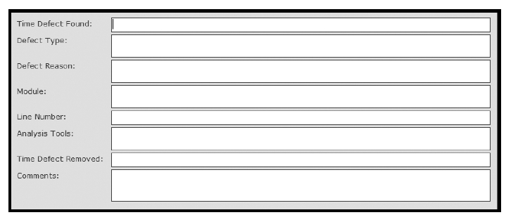Figure 17: Form used to input errors into the database

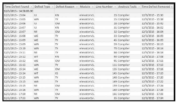Figure 18: Excerpt from the table holding the errors discovered in run one of testing the elevator controller

Table 8: The final results for our benchmark programs

Error Rate	Program Tested	Data Model	S	Pseudo Adjusted R-Squared
High	Automated Door	Base Exponential	5.6586	0.4267
		Exponential	4.8513	0.5957
		Modified Exponential	4.7571	0.5789
		Multinomial Exponential	3.8516	0.7452
	Security System	Base Exponential	5.6457	0.6351
		Exponential	4.7965	0.7297
		Modified Exponential	4.7162	0.7201
		Multinomial Exponential	N/A	N/A
	Streetlight	Base Exponential	4.4259	0.5411
		Exponential	3.7957	0.6425
		Modified Exponential	3.9823	0.6356
		Multinomial Exponential	3.8650	0.6293
	Tollbooth	Base Exponential	5.2394	0.4518
		Exponential	4.9228	0.5655
		Modified Exponential	4.8191	0.5316
		Multinomial Exponential	4.5043	0.6149
	Vending Machine	Base Exponential	2.4275	0.8491
		Exponential	1.7077	0.9306
		Modified Exponential	1.8919	0.9248
		Multinomial Exponential	1.7077	0.9306
Low	Automated Door	Base Exponential	4.5366	0.4411
		Exponential	3.8664	0.6091
		Modified Exponential	4.1704	0.5866
		Multinomial Exponential	3.9120	0.6091
	Security System	Base Exponential	2.6590	0.8513
		Exponential	1.5579	0.9488
		Modified Exponential	1.5175	0.9457
		Multinomial Exponential	N/A	N/A
	Streetlight	Base Exponential	2.6988	0.7028
		Exponential	2.4116	0.7594
		Modified Exponential	2.3674	0.7488
		Multinomial Exponential	2.4524	0.7512
	Tollbooth	Base Exponential	3.0550	0.6349
		Exponential	1.9577	0.8601
		Modified Exponential	2.1923	0.8496
		Multinomial Exponential	1.1234	0.9539
	Vending Machine	Base Exponential	2.4878	0.6034
		Exponential	1.2017	0.8980
		Modified Exponential	1.3557	0.8902
		Multinomial Exponential	0.8980	1.2017

As we can see from the results, there is a definitive increase in the model fitment compared to the base, unmodified exponential model when the outliers are removed. The results show that in some cases the standard exponential model fits the data the best, in others the modified exponential, and in others the multinomial exponential. For the Vending Machine results, in both the high and low error rate results, the multinomial is the base exponential, as the best exponent has only the “x” term in it. From the results we can see that there is not any way to predict at this time which model works best for which rate, as each group has examples where each is the best for that program. In the case of the Security System, the multinomial could not be processed for both error rates, as the multinomial equation that fit best diverged to infinity when used as the exponent to an exponential.

12. Conclusion

The work presented here shows our complete design and testing process used in creating an initial benchmark suite for software reliability. Error analysis discovery with formal methods was shown to be more widely applicable than originally reported in [1], as we showed that errors could also be found by ATPs in the proof, not just the specification. We illustrated our RNG testing and random error generation that previously was mentioned in [2] but was not demonstrated in that work. This was utilized to help enhance our results in [3] and expand our tested programs. This expanded program suite illustrates that software errors, using a proper development process, can be shown to be modeled statistically similar to hardware. We have shown through the removal of outliers that the results can be improved further still. This development process and the full results set a benchmark, so other development processes can be researched and even better software analysis can be achieved.

13. Future Work

Based on the work presented here, the first major area of expansion is the benchmarks themselves. We have shown the development and testing process allows small scale software programs to meet the statistical models that were originally theorized. This is great for embedded systems, but the process may be applicable to large system on chip solutions, or even large scale, big data applications. To begin this expansion, we will develop larger, more complex versions of the six benchmark programs already developed to see if the results hold when scaled up.

Similar to this area is the need to improve the development process with good, well developed software modules. In hardware, most systems are incorporated with ICs that come from manufacturers with known reliability. The same should be true of software. If modules have already been vetted through the development process, then they should be correct and accurate, allowing their reuse as a black box, and improving the error results of a new system prior to testing. This would be similar to pulling an IC of AND or NOT gates from the parts bin, knowing what it does and expecting it to work, without seeing the intricacies inside the black box.

The other side of safety critical systems is determining trust. Work in this space has looked into ways of showing trust for both hardware and software. Our development process could aid in this area, being twofold with reliability, if measures of security and trust can be incorporated into the formal method specification. In the future we will use the original elevator specification and redesign it, incorporating new security measures, while maintaining our current reliability measures. We will attempt to show the proofs can be developed to show security and reliability in one step, allowing for their incorporation from the beginning of design.

One final area of expansion is the integration of the software designed with this process into a targeted application. This requires further improvement of the software reliability in the system. Unlike hardware, which can use redundancy of circuitry to improve reliability, copying software with an undiscovered bug just propagates that bug to all versions. One solution may be to develop a hardware based monitor, possibly with machine learning, to determine when a software anomaly has been seen, and correct it. AI could be trained on the state and inputs of the system to know what outputs should be provided, and if the wrong output is generated from a known state, then a safety protocol could be enacted for a trusted system, or just replaced with the correct value for a non-critical system.

Conflict of Interest

The authors declare no conflict of interest.

Acknowledgments

The authors would like to thank L-3 Fuzing and Ordnance Systems. A portion of this work was funded in part by their generous grant.

1.  J. Lockhart, C. Purdy, and P. A. Wilsey, “The use of automated theorem proving for error analysis and removal in safety critical embedded system specifications,” in 2017 IEEE National Aerospace and Electronics Conference (NAECON), June 2017, pp. 358–361.
2.  J. Lockhart, C. Purdy, and P. A. Wilsey, “Error analysis and reliability metrics for software in safety critical systems,” in 2016 IEEE 59th International Midwest Symposium on Circuits and Systems (MWSCAS), Oct 2016, pp. 1–4.
3.  J. Lockhart, C. Purdy, and P. A. Wilsey, “Error analysis and reliability metrics for software in safety critical systems,” in 2018 IEEE 61st International Midwest Symposium on Circuits and Systems (MWSCAS), 2018.
4.  A. Mishchenko, S. Chatterjee, and R. Brayton, “Dag-aware aig rewriting: a fresh look at combinational logic synthesis,” in 2006 43rd ACM/IEEE Design Automation Conference, July 2006, pp. 532–535.
5.  C. Albrecht, “Iwls 2005 benchmarks,” ””, Tech. Rep., Jun 2005.
6.  J. Cong and K. Minkovich, “Optimality study of logic synthesis for lut-based fpgas,” Computer-Aided Design of Integrated Circuits and Systems, IEEE Transactions on, vol. 26, no. 2, pp. 230–239, Feb 2007.
7.  Static & Formal Verification. [Online]. Available: https://www.synopsys.com/verification/ static-and-formal-verification.html (Accessed 2017-3-17).
8.  A. J. Hu. Formal hardware verification with bdds: An introduction. [Online]. Available: https://www.cs.ox.ac.uk/ files/4309/97H1.pdf (Accessed 2017-4-22).
9.  A. J. Hu, “Formal hardware verification with bdds: an introduction,” in 1997 IEEE Pacific Rim Conference on Communications, Computers and Signal Processing, PACRIM. 10 Years Networking the Pacific Rim, 1987-1997, vol. 2, Aug 1997, pp. 677–682 vol.2.
10.  Arvind, N. Dave, and M. Katelman, “Getting formal verification into design flow,” in Proceedings of the 15th International Symposium on Formal Methods, ser. FM ’08. Berlin, Heidelberg: Springer-Verlag, 2008, pp. 12–32. [Online]. Available: http://dx.doi.org/10.1007/978-3-540-68237-0 2
11.  Arvind, N. Dave, and M. Katelman. Getting Formal Verification into Design Flow. [Online]. Available: http://people.csail.mit.edu/ndave/Research/fm 2008.pdf (Accessed 2017-4-22).
12.  J. Markoff. (2016) Moore’s law running out of room, tech looks for a successor. [Online]. Available: http://tinyurl.com/MooresLawOutOfRoom (Accessed 2016-5- 6).
13.  J. Hruska. (2016, July) Moore’s law scaling dead by 2021, to be replaced by 3d integration. [Online]. Available: https://tinyurl.com/EXT-MooresLaw (Accessed 2018-3-17).
14.  R. Smith. (2015) Amd dives deep on high bandwith memory – what will hmb bring amd. [Online]. Available: http: //www.anandtech.com/show/9266/amd-hbm-deep-dive (Accessed 2016-4-29).
15.  AMD. (2015) High bandwidth memory — reinventing memory technology. [Online]. Available: http://www.amd. com/en-us/innovations/software-technologies/hbm (Accessed 2016-4-29).
16.  J. Hruska. (2017, July) Mit develops 3d chip that integrates cpu, memory. [Online]. Available: https: //tinyurl.com/EXT-MIT-3D-Chip (Accessed 2018-3-17).
17.  H. Knight. (2017, July) New 3-d chip combines computing and data storage. [Online]. Available: http://news.mit.edu/2017/ new-3-d-chip-combines-computing-and-data-storage-0705 (Accessed 2018-3-17).
18.  M. Suri, D. Querlioz, O. Bichler, G. Palma, E. Vianello, D. Vuillaume, C. Gamrat, and B. DeSalvo, “Bio-inspired stochastic computing using binary cbram synapses,” IEEE Transactions on Electron Devices, vol. 60, no. 7, pp. 2402–2409, July 2013.
19.  K. Alrawashdeh and C. Purdy, “Fast hardware assisted online learning using unsupervised deep learning structure for anomaly detection,” in International Conference on Information and Computer Technologies (ICICT 2018). IEEE, 2018, p. In Press.
20.  T. Griggs and D. Wakabayashi. (2018, March) How a selfdriving uber killed a pedestrian in arizona. [Online]. Available: https://tinyurl.com/ybvcgfu4 (Accessed 2018-3-28).
21.  R. Marosi. (2010) Runaway prius driver: ’i was laying on the brakes but it wasn’t slowing down’. [Online]. Available: http://articles.latimes.com/2010/mar/10/business/ la-fi-toyota-prius10-2010mar10 (Accessed 2014-1-26).
22.  A. Haxthausen, “An introduction to formal methods for the development of saftey-critical applications,” Technical Univeristy of Denmark, Lyngby, Denmark, Tech. Rep., August 2010.
23.  G. Finzer. (2014) How many defects are too many? [Online]. Available: http://labs.sogeti.com/ how-many-defects-are-too-many/ (Accessed 2016-4-29).
24.  V. R. Basili and B. T. Perricone, “Software errors and complexity: An empirical investigation,” Commun. ACM, vol. 27, no. 1, pp. 42–52, Jan. 1984. [Online]. Available: http://doi.acm.org/10.1145/69605.2085
25.  J. D.Musa, “A theory of software reliability and its application,” IEEE Transactions on Software Engineering, vol. SE-1, no. 3, pp. 312–327, Sept 1975.
26.  J. D. Musa and A. F. Ackerman, “Quantifying software validation: when to stop testing?” IEEE Software, vol. 6, no. 3, pp. 19–27, May 1989.
27.  S. Yamada, Software reliability modeling: fundamentals and applications. Springer, 2014. [Online]. Available: https://link. springer.com/content/pdf/10.1007/978-4-431-54565-1.pdf
28. S. Yamada and S. Osaki, “Reliability growth models for hardware and software systems based on nonhomogeneous poisson processes: A survey,” Microelectronics Reliability, vol. 23, no. 1, pp. 91 – 112, 1983. [Online]. Available: http://www. sciencedirect.com/science/article/pii/0026271483913720
29.  S. Yamada, Stochastic Models in Reliability and Maintenance. Berlin, Heidelberg: Springer Berlin Heidelberg, 2002, ch. Software Reliability Models, pp. 253–280. [Online]. Available: http://dx.doi.org/10.1007/978-3-540-24808-8 10
30.  H. D. Drake and D. E. Wolting, “Reliability theory applied to software testing,” Hewlett-Packard Journal, vol. 38, pp. 35–39, 1987.
31.  RTCA and EUROCAE, “Software considerations in airborne systems and equipment certification,” RTCA, Inc.,Washington, D.C., USA, Tech. Rep., 1992.
32.  Federal Aviation Administration, “Advisory circular 20-174,” U.S. Department of Transportation, Tech. Rep., 2011. [Online]. Available: https://www.faa.gov/documentLibrary/media/ Advisory Circular/AC 20-174.pdf
33.  J. Lockhart, C. Purdy, and P.Wilsey, “Formal methods for safety critical system specification,” in 2014 IEEE 57th International Midwest Symposium on Circuits and Systems (MWSCAS), Aug 2014, pp. 201–204.
34.  M. Popovic, V. Kovacevic, and I. Velikic, “A formal software verification concept based on automated theorem proving and reverse engineering,” in Engineering of Computer-Based Systems, 2002. Proceedings. Ninth Annual IEEE International Conference and Workshop on the, 2002, pp. 59–66.
35.  J. Rushby, “Harnessing disruptive innovation in formal verification,” in Software Engineering and Formal Methods, 2006. SEFM 2006. Fourth IEEE International Conference on, Sept 2006, pp. 21–30.
36.  W. Visser, K. Havelund, G. Brat, and S. Park, “Model checking programs,” in Automated Software Engineering, 2000. Proceedings ASE 2000. The Fifteenth IEEE International Conference on, 2000, pp. 3–11.
37.  Lemma 1, “Getting started,” in ProofPower: Tutorial. Berkshire, United Kingdom: Lemma 1 Ltd, 2006, ch. 1, pp. 5–10.
38.  H. Ganzinger and V. Sofronie-Stokkermans, “Chaining techniques for automated theorem proving in many-valued logics,” in Multiple-Valued Logic, 2000. (ISMVL 2000) Proceedings. 30th IEEE International Symposium on, 2000, pp. 337–344.
39.  C. Morgan, “Methods for automated theorem proving in nonclassical logics,” Computers, IEEE Transactions on, vol. C-25, no. 8, pp. 852–862, Aug 1976.
40.  A. A. Larionov, E. A. Cherkashin, and A. V. Davydov, “Theorem proving software, based on method of positively-constructed formulae,” in MIPRO, 2011 Proceedings of the 34th International Convention, May 2011, pp. 965–968.
41.  M. Kaufmann and J. S. Moore, “Some key research problems in automated theorem proving for hardware and software verification,” in RACSAM. Revista de la Real Academia de Ciencias Exactas, Fisicas y Naturales. Serie A. Matematicas, vol. 98, no. 1, Oct 2004, pp. 181–195.
42.  J. Bowen and V. Stavridou, “Safety-critical systems, formal methods and standards,” Software Engineering Journal, vol. 8, no. 4, pp. 189–209, Jul 1993.
43.  E. M. Clarke and J. M. Wing, “Formal methods: State of the art and future directions,” ACM Comput. Surv., vol. 28, no. 4, pp. 626–643, Dec 1996.
44.  Z. Li, S. Lu, S. Myagmar, and Y. Zhou, “Cp-miner: finding copy-paste and related bugs in large-scale software code,” IEEE Transactions on Software Engineering, vol. 32, no. 3, pp. 176–192, March 2006.
45.  S. Morasca, “A probability-based approach for measuring external attributes of software artifacts,” in 2009 3rd International Symposium on Empirical Software Engineering and Measurement, Oct 2009, pp. 44–55.
46.  A. Varshney, R. Majumdar, C. Choudhary, and A. Srivastava, “Role of parameter estimation & prediction during development of software using srgm,” in Reliability, Infocom Technologies and Optimization (ICRITO) (Trends and Future Directions), 2015 4th International Conference on, Sept 2015, pp. 1–6.
47.  D. Tang and M. Hecht, “Evaluation of software dependability based on stability test data,” in Fault-Tolerant Computing, 1995. FTCS-25. Digest of Papers., Twenty-Fifth International Symposium on, June 1995, pp. 434–443.
48.  Y. Tamura and S. Yamada, “Reliability analysis based on a jump diffusion model with two wiener processes for cloud computing with big data,” Entropy, vol. 17, no. 7, pp. 4533–4546, 2015. [Online]. Available: http://www.mdpi.com/1099-4300/17/7/4533
49.  S. Yamada and M. Yamaguchi, “A method of statistical process control for successful open source software projects and its application to determining the development period,” International Journal of Reliability, Quality and Safety Engineering, vol. 23, no. 05, p. 1650018, 2016. [Online]. Available: https://www.worldscientific.com/doi/abs/10.1142/ S0218539316500182
50.  ISO/IEC, “Information technology: Z formal specification notation : syntax, type system, and semantics,” International Organization for Standardization and International Electrotechnical Commission, Geneva, Switzerland, Standard 13568, 2002.
51.  ISO/IEC, “Information technology, programming languages, their environments and system software interfaces, vienna development method, specification language,” International Organization for Standardization and International Electrotechnical Commission, Geneva, Switzerland, Standard 13817-1, 1996.
52.  M. Huth and M. Ryan, “Propositional logic,” in Logic in Computer Science: Modelling and Reasoning about Systems, 1st ed. Cambridge, United Kingdom: Cambridge University Press, 2000, ch. 1, pp. 1–88.
53.  J. Davies and J. Woodcock, “Propositional logic,” in Using Z: Specification, Refinement, and Proof, 1st ed. Hertfordshire, United Kingdom: Prentice Hall Europe, 1996, ch. 2, pp. 9–26.
54.  M. Huth and M. Ryan, “Predicate logic,” in Logic in Computer Science: Modelling and Reasoning about Systems, 1st ed. Cambridge, United Kingdom: Cambridge University Press, 2000, ch. 2, pp. 90–146.
55.  J. Davies and J. Woodcock, “Predicate logic,” in Using Z: Specification, Refinement, and Proof, 1st ed. Hertfordshire, United Kingdom: Prentice Hall Europe, 1996, ch. 3, pp. 37–2012 44.
56.  J. M. Spivey, “Basic concepts,” in Understanding Z: A Specification Language and its Formal Semantics, 1st ed. New York, New York: Cambridge University Press, 1988, ch. 2, pp. 18–24.
57.  J. Davies and J. Woodcock, “Sets,” in Using Z: Specification, Refinement, and Proof, 1st ed. Hertfordshire, United Kingdom: Prentice Hall Europe, 1996, ch. 5, pp. 57–72.
58.  J. M. Spivey, “Studies in z style,” in Understanding Z: A Specification Language and its Formal Semantics, 1st ed. New York, New York: Cambridge University Press, 1988, ch. 5, pp. 98–113.
59.  Lemma 1, “Solutions to exercises,” in ProofPower: Z Tutorial. Berkshire, United Kingdom: Lemma 1 Ltd, 2006, ch. 8, pp. 143–149.
60.  H. Pishro-Nik. (””, ””) 11.1.4 nonhomogeneous poisson processes. [Online]. Available: https://tinyurl.com/yb5kbspn (Accessed 2018-12-7).
61.  K. Siegrist. (””, ””) 6. non-homogeneous poisson processes. [Online]. Available: https://tinyurl.com/yc9y9vch (Accessed 2018-12-7).
62.  MIT OpenCourseWare. (2011, Spring) Chapter 2 poisson processes. [Online]. Available: https://tinyurl.com/ycg6r3n4 (Accessed 2018-12-7).
63.  NIST. (””, ””) 8.1.7.2. non-homogeneous poisson process (nhpp) – power law. [Online]. Available: https: //tinyurl.com/yclorwqd (Accessed 2018-12-7).
64.  S. Yamada, “Software reliability models,” in Stochastic Models in Reliability and Maintenance, S. Osaki, Ed. Springer Berlin Heidelberg, 2002, pp. 253–280.
65.  V. Putz. (2000) The personal software process: an independent study. [Online]. Available: http://www.nyx.net/_vputz/ psp index/book1.html (Accessed 2013-10-30).
66.  H. Watts, “The personal software process (psp),” Software Engineering Institute, Carnegie Mellon University, Pittsburgh, PA, Tech. Rep. CMU/SEI-2000-TR-022, 2000. [Online]. Available: http://resources.sei.cmu.edu/library/asset-view.cfm? AssetID=5283
67.  V. Putz. (2000) Program 1a. [Online]. Available: http://www.nyx.net/_vputz/psp index/x341.html (Accessed 2017-02-16).
68.  V. Putz. (2000) Program 2a: Simple loc counter. [Online]. Available: http://www.nyx.net/_vputz/psp index/x1547.html (Accessed 2017-01-26).
69.  V. Putz. (2000) Chapter 2. lesson 2: Planning and measurement. [Online]. Available: http://www.nyx.net/_vputz/psp index/ c1028.html (Accessed 2013-10-30).
70.  D. E. Knuth, The Art of Computer Programming, Vol. 1, 3rd ed. Addison-Wesley, 1997.
71.  D. E. Knuth, The Art of Computer Programming, Volume 2: Seminumerical Algorithms, 3rd ed. Addison-Wesley, 1998.
72.  Marsaglia, “Note on a proposed test for random number generators,” IEEE Transactions on Computers, vol. C-34, no. 8, pp. 756–758, Aug 1985.
73.  P. L’Ecuyer and R. Simard, “Testu01 a software library in ansi c for emperical testing of random number generators,” D´epartement d’Informatique et de Recherche Op´erationnelle Universit´e de Montr´eal, Tech. Rep., 2013. [Online]. Available: http://simul.iro.umontreal.ca/testu01/ guideshorttestu01.pdf
74.  P. L’Ecuyer and R. Simard, “Testu01: A c library for empirical testing of random number generators,” ACM Trans. Math. Softw., vol. 33, no. 4, Aug. 2007. [Online]. Available: http://doi.acm.org/10.1145/1268776.1268777
75.  M. E. O’Neill, “Pcg: A family of simple fast space-efficient statistically good algorithms for random number generation,” Harvey Mudd College, Claremont, CA, Tech. Rep. HMC-CS-2014-0905, Sep. 2014.
76.  F. Neugebauer, I. Polian, and J. P. Hayes, “Building a better random number generator for stochastic computing,” in 2017 Euromicro Conference on Digital System Design (DSD), Aug 2017, pp. 1–8.
77.  J. Lockhart, K. A. Rawashdeh, and C. Purdy, “Verification of random number generators for embedded machine learning,” in 2018 IEEE National Aerospace and Electronics Conference (NAECON), In Press 2018.
78.  UCLA: Institute for Digital Research and Education. (2011) Faq: What are pseudo r-squareds? [Online]. Available: https://stats.idre.ucla.edu/other/mult-pkg/faq/general/ faq-what-are-pseudo-r-squareds/ (Accessed 2018-6-9).

(Click Here)

(Click Here)