1. Introduction

Problems in video prediction (spatiotemporal prediction) are important in both research and industry. Examples include human action recognition [1], spread of infections, medical predictions [2], weather forecast prediction [3], and autonomous car video prediction systems [4,5].

Spatiotemporal (e.g. video) datasets are challenging to predict due to the spatial and temporal information which the datasets carry through time. In sequence prediction problems, the prediction at the current step depends primarily on the previous history. Making a near future prediction requires an computational tool that is able to discover both the long and short-term dependencies in the data. Initially, recurrent neural networks (RNN) [6] were proposed to model data which was sequential in nature. However, straightforward RNNs have major drawbacks. RNNs suffer from the vanishing/exploding gradient problem which prevents them from learning long-term data dependencies [7–9]. There are several gate-based RNN models that attempt to solve this classic problem. These include the long short-term memory unit (LSTM) [7], peephole LSTM [10], gated recurrent unit (GRU) [10], and minimal recurrent unit (MRU) [11].

This paper studies the LSTM architecture as an attractive architecture architecture to perform spatiotemporal (video) prediction. In addition, Gref et al. [12] empirically showed that the LSTM is the most efficient recurrent architecture to solve for speech recognition, handwriting recognition, and polyphonic music modeling [12]. The LSTM has the highest number of gates compared with other gated units [9–11]. Furthermore, the choice of the activation function for gate and nongate units within the LSTM has an essential effect on the the LSTM’s function [12].

This work studies gate activations and non-gate activations within the LSTM architecture. In most APIs the gate activations and non-gate activations are known as recurrent activations and unit activations, respectively. To solve image and video related problems, different convolution-based models are used such as in Kalchbrenner et al [13], Elsayed et al. [5], Lotter et al. [4], Finn at al. [14], and Wang et al. [15]. However, the most widely used architecture for video prediction to-date is the convolution LSTM. Hence, we performed our experiments on a convolution-based LSTM (convolutional LSTM) network model [4]. We studied the effect of different gate activation and unit activation functions through the learning process of the convolutional LSTM architecture [3]. Our experiments use the convolutional LSTM found in the Keras deep learning framework [16]. Training was performed on the moving MNIST dataset as the most commonly used benchmark for video prediction problems [17].

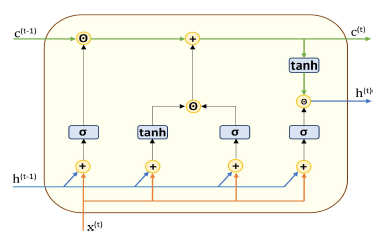Figure 1: The unrolled LSTM architecture. The memory-state and output lines are time-evolving and labelled c and h, respectively. The CEC is indicated by the plus sign on the c line. The level of description is coarse enough so that this could either depict a standard LSTM or a convolutional LSTM.

In our empirical study, we worked with a model than what was needed for optimal prediction. Specifically, it had fewer parameters. This reduction allows us to more clearly see the effect of gate and unit activations on the convLSTM model without contamination by influences of other high-effect parameters. For example, it avoids saturation effects on the model accuracy which helps to see changes in activation function effects [18]. Our study compares different activation functions on a simple convolutional LSTM model for spatiotemporal (video) prediction task. We investigated the responsibilities of the convolutional LSTM gates and unit activations over the training process. Furthermore, we found the most appropriate function to be applied for the gates and for the unit activation for solving video prediction problem.

2. Convolutional LSTM

The LSTM [7] is the first gate-based recurrent neural network. As noted earlier, it was motivated by the need to mitigate the vanishing gradient problem and did so by using the principle underlying a constant error carousel (CEC) [7] to improve the learning of long-term dependencies. This was implemented by adding a memory-state line to the architecture (Figure 1). This memory-state line can retain (remember) the recurrent values over arbitrary time intervals. Gres et al. [8] added a forget gate to the LSTM cell to allow information to be removed from (forgotten) the memory-state line. This gate was trainable so that the module could learn when stored information was no longer needed. Gers et al. [10] improved the design by adding so-called peephole connections from the memory cell to the LSTM gates. The peephole connections enable the memory line to exert control over the activation of all three of the gates. This helps the LSTM block to avoid vanishing gradients and also helps learning of precise timing in conjunction with Constant Error Carousel (CEC) [8]. The CEC is the key ingredient mitigate the vanishing gradient problem.

LSTMs are used in several application areas including speech recognition [19,20], language modeling [21], sentiment analysis [22], music composition [23], signal analysis [24], human action recognition [1], image caption generation [25], and video prediction [3,4,17,26].

The convolutional LSTM (convLSTM) was introduced in 2015 by Shi et al [3] for weather precipitation forecast prediction task. This is an enhancement to the LSTM discussed previously. The crucial change is that the data within the module takes the form of a multichannel 2D feature map (image stack). The convLSTM improves predicted video on data sets of evolving precipitation maps compared to the non-convolutional LSTM. Apparently, it captures spatiotemporal correlations better than non-the standard variant [3,17].

An unrolled convLSTM module in Figure 1 can be either standard or convolutional because it does not make the relevant internal operations and weights explicit. Like the standard LSTM, the architecture has three gates indicated by the activation functions labeled σ. These are the forget, input, and output gates [9]. There are two non-gate units which are labeled with tanh activation functions. The convLSTM gates (input, forget, and output) have the ability to multiplicatively attenuate the outputs of tanh units and the value on the c^(t−1) line. The forget gate attenuates information deemed unnecessary from the previous cell memory state c^(t−1). h^(t−1) is the convLSTM cell output at time t − 1, and h^(t) is the output of the convLSTM cell at time t. x^(t) is the current video frame target at time t. c^(t−1) and c^(t) are the memory cell states at consecutive times.

The following equations calculate all of the gate and the unit values based on the Gers et al. [8] LSTM combined the convolutional model of Shi et al. [3]. These operations should be compared with Figure 2.

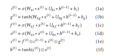The the input, forget, and output gate activations s are denoted i^(t), f ^(t), and o^(t). σ denotes logsig. The gates have activation values falling in the interval [0,1] where 1 means completely open and 0 means completely closed. g^(t), is the current input. c^(t) represents the current memory module state. h^(t) represents the current output. b_i, b_g, b_f , and b_o are biases for the respective gate. W’s and U’s are the feedforward and

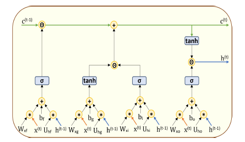Figure 2: The unrolled convLSTM architecture at the arithmetic operation level. This rendering makes convolution operations and weights

explicit and should be compared with Equation Set 1.

recurrent weights, respectively. “” denotes elementwise multiplication, and “∗” denotes the convolution operator.

Figure 2 shows the arithmetic operational level of the convLSTM architecture where the convLSTM components and their corresponding weights are shown explicitly.

3. Activation Functions

As explained earlier, gate units usually have sigmoid

(range [0,1]) activation functions and non-gated units usually have tanh activation functions. This paper studies the effects of using different activation functions for these units. This section reviews the most common activation functions used. All of the functions discussed are nonlinear.

Figure 3: The curve of the logsig (σ) function.

3.1. Logsig Function

The logistic sigmoid (logsig) function [27] is shown in Figure 3. It is given by the following equation:

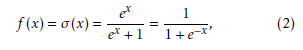The logsig is commonly denoted by σ(x), where x ∈ (−∞,∞) and σ(x) ∈ (0,1). The logsig is historically common in network models because it intuitively represents the firing rate of a biological neuron. The logsig is still used in recurrent models for gating purposes. The input value is usually known because it appears in the feedforward sweep of the network. Because of this, its derivative can be computed efficiently as shown in (3).

3.2. Hard-Sigmoid Function

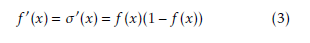
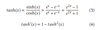
The hard-sigmoid (hardSig) function is considered a noisy activation function. HardSig approximates logsig function by taking the first-order Taylor expansion around zero and clipping the result according to function’s range [0,1]. Hardsig appears in Figure 4 and is calculated as follows:

This function allows a crisp decision for the gradient during function saturation phase to be either fully on or fully off. In the non-saturation range near zero, hardSig is linear. This helps avoid vanishing gradients [28].

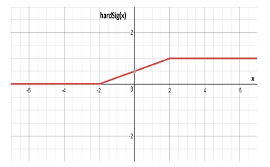Figure 4: The curve of the hardSig function.

3.3. Hyperbolic Tangent Function

tanh is a saturating activation function. It is typically used as the recurrent activation function in RNNs [6].

In some cases, tanh is considered as cheaper for gradient evaluation in comparison to the logsig function. The function graph appears in Figure 5 and is specified by (5):

A convenient property of the tanh activation function is that calculating its first derivative from a known input value is easy as seen in Eqn. (6).

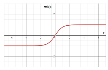Figure 5: The curve of the Hyperbolic Tangent function.

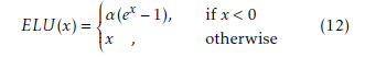
3.4.  SoftSign Function

The SoftSign function was introduced in [29]. Its grahp is given in Figure 6 and is specified by:

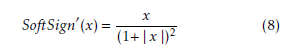
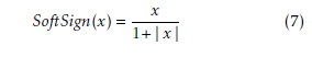The SoftSign function range is (−1,1) and the function domain is x ∈ (−∞,∞). The first derivative of SoftSign also can be evaluated simply as the following:

SoftSign is an alternative function to hyperbolic tanh. In comparison to tanh, it does not saturate as quickly, improving its robustness to vanishing gradients.

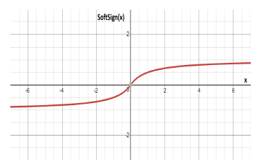Figure 6: Curve of the SoftSign function.

3.5. ReLU Function

The rectified linear unit (ReLU) is very efficient compared to other activation functions. It was proposed in [30]. For x ≥ 0 it is the identity function and appears in Figure 7. ReLU is defined by:

Its has domain x ∈ (−∞,∞) and range [0,∞).

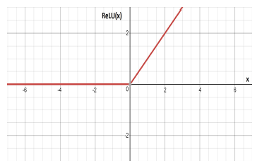Figure 7: The curve of the ReLU function.

3.6.  SoftPlus Function

The SoftPlus function (Figure 8) was proposed in [31]. It modifies the ReLU by applying a smoothing effect [29] and is defined:

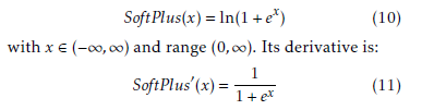Like the SoftSign function, the SoftPlus function is used only in specific applications.

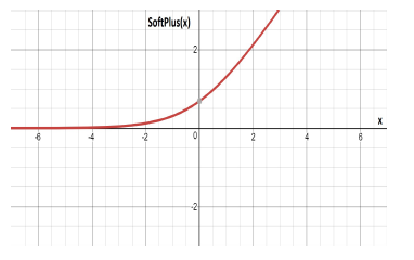Figure 8: The curve of the SoftPlus function.

3.7. ELU Function

The exponential linear unit (ELU) was introduced in [32] to avoid a zero derivative for negative input values.

The ELU achieved better classification accuracy than ReLUs [32] and is defined by:

Its domain and range is (−∞,∞). Assuming that α = 1, its graph is shown in Figure 9 .

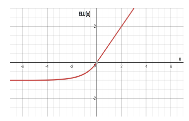Figure 9: The curve of the ELU function.

3.8.  SELU Function

The scaled exponential linear unit (SELU) an ELU function modified with two hyperparameters. Its definition follows:

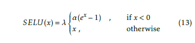Its domain is the same as the ELU function, but its range is limited to −(λα,∞). λ and α are hyperparameters that depend on the mean and variance of the training data. If the data is normalized to µ = 0 and σ = 1, then λ = 1.0507 and α = 1.6732 whose graph appears in Figure 10.

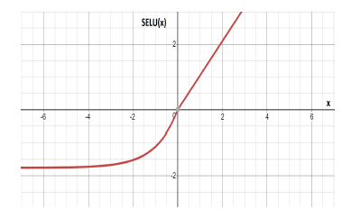Figure 10: The curve of the SELU function.

The first derivative of SELU is calculated as shown below:

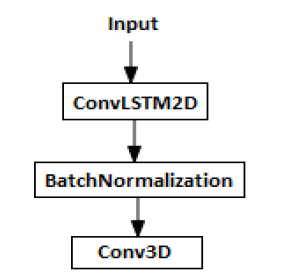Figure 11: The model architecture used in our experiments.

4. Experiments and Results

This section the results of comparing different activation functions for both the gate units and non-gate units. We chose the functions described in the previous section. They are commonly available in deep learning frameworks. We explore the question of which activation function is best as a gate activation and which is best as a unit activation for convolutional LSTMs in an unsupervised context. Moreover, we want to understand the differential behavior of the gate and non-gate units as a result of training.

We calculated several measures: training loss, validation loss, elapsed training time, and appearance of the predicted video frames compared with ground truth. We did our experiment and analysis on the moving MNIST [17] as explained in the introduction. The moving MNIST dataset consists of 10,000 different video sequences. Each sequence has a length of 20 frames. Each frame is 64 × 64 pixels and contains two randomly selected handwritten digits from the standard 28 × 28 MNIST dataset. The two digits move randomly within the frame [17].

4.1. Framework

Our framework uses Shi’s et al. [3] convLSTM. Because we had limits on our computing power, our test were serendipitously performed using a small model with insufficient learning capacity for fully accurate predictions. However, this did let us more clearly see the effects of the activation function manipulations. The reduced capacity models helped us avoid ceiling effects so that we could see differential performances in the activation functions.

The model is implemented using the Keras API [16] and appears in Figure 11. It consists of three layers. The first layer is a convLSTM with 40 size 3×3 kernels.

The next layer is batch normalization. Finally, we used 3 × 3 × 3 kernel to get the video output shape. Table 1 provides details of the model parameters.

Table 1: Description of the proposed model architecture used in this study. Layer (type) Output Shape Param Number ConvLSTM2D (None, None, 64, 64, 10) 4000 Batch Normalization (None, None, 64, 64, 10) 40 Conv3D (None, None, 64, 64, 1) 271 Total params 4,311 Trainable params 4,291 Non-trainable params 20

The Adam optimizer [33] was used with initial learning rate r = 0.001, β₁ = 0.9, β₂ = 0.999. The cost function was MSE [34].

Each input was a 20-frame video randomly sampled from moving MNIST [17]. As previously mentioned, the amount of input data is 10,000 videos each of length 20 frames. We used 9,500 for training and 500 for validating.

The task is proposed for sequence to sequence video prediction. A sequence of five future frames were predicted using the previous five frame sequence. Because of the reduced learning capacity mentioned at the beginning of this section, the trained network could predict only the two temporally closed frames clearly and the rest were unclear because of the reduced learning capacity in the model.

We used an Intel(R) Core i7 − 7820HK, 32GB RAM, and a GeForce GTX 1080 GPU. Training was for ten epochs in each experiment. In each epoch, we fit 475 batches where each batch size was set to 20 for our model experiments. All parameters were held constant over all experiments except for the recurrent activation function that was being tested.

4.2. Results

Our results pertain to the relative performance of varied activation functions for gate and non-gate units.

4.2.1        Results for Gate Activation Functions

For a fair comparison of different gate activation functions, we only changed the gate activation functions and preserved the remaining parameters with the same initializations and values during each experiment. The gate effects were studied collectively because we used the default convolutional LSTM module in found in the Keras API. The API allowed us to change all the gate functions at once (not each gate separately) for setting up an experiment.

For this experiment, the gate activation functions apply to all three gates gates described in Eqns 1a, 1c, and 1d. Accordingly, only functions with range (0,1) are eligible. Thus, this experiment only compared the logsig and hardSig functions.

Table 2 shows the performance results, including average elapsed training time (in minutes), MSE loss (Loss-MSE) for training, validation loss (Val-loss-MSE), percent accuracy (Accuracy) for n = 3, and the standard error (SE) for training loss (n = 3). The elapsed training time using the hardSig activation is higher than the logsig function by about ten percent. We are not sure why this happens. In Table 2, both logsig and hardSig have nearly exactly the same MSE and MAE.

Figure 12 shows the training and validation loss for the logsig and hardSig activation functions. From the figure, one can also see that the loss average difference between the training and validation runs using the hardSig function is smaller than the logsig function.

We also examined the differences between the accuracy of both training and validation runs using the logsig versus hardSig functions. The average (n = 3 for all data points) accuracy values for each function appear in Figure 13. Blue represents training and yellow represents validation accuracy. Both logsig and hardSig functions have similar validation and training accuracy It is also temporally time. The hardSig shows a more comparable accuracy among the training and validation curves. Moreover, hardSig curve does not contain frequent validation accuracy drops down as in logsig curve.

Figure 14 visually shows the prediction results for both the sigmoid and hardSig gate activations of the model. The first row shows ground truth. The two rows below show predictions using the logsig versus hardSig gate activation functions. Both logsig and hardSig are comparable. From the figure, both functions show that the model attempts to learn the digit movement trajectories as shown in each of the prediction frames. The ‘double exposure’ appearance indicates that the prediction retains the object’s previous location within the predicted frame. Despite the double exposure look, digit shape is preserved. Moreover, the hardSig function shows better prediction accuracy than the sigmoid. This agrees with the Gulcehre et al. [28] theory stating that noisy activation functions are better than their non-noisy counterparts.

This experiment suggests the gate activation functions of the convolutional LSTM play a role learning the movement trajectories.

4.2.2        Results for Non-gate Activations

Our second experiment analyzes which activation function is best to use for non-gate units (input-update and output activation) as seen in Eqns. 1b and 1f. We applied the same setup and initialization as in the first experiment except that we retained all the convLSTM parameters. Only the set of possible unit activation functions were manipulated. Gate activations were

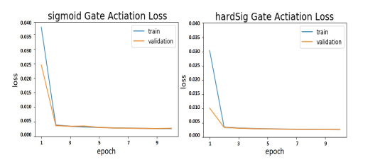Figure 12: Training and validation loss for each gate activation function over each training epoch. In the left figure, all three gate units used the logsig activation. In the right figure, all three gate units used the hardSig activation function.

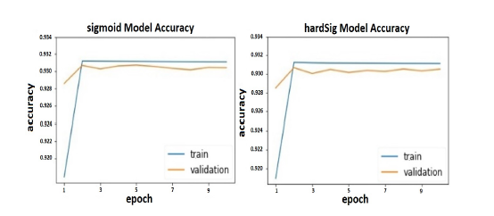Figure 13: Training and validation accuracy for each gate activation function over each training epoch.

Table 2: Gate Activation Effect on the ConvLSTM Training Process.

Activation function			Training Results
	Time	Loss	Val-loss	Mean Absolute	Accuracy	SE
	(Minutes)	(MSE)	(MSE)	Error (MAE)	(Percentage)	(Loss)
sigmoid	20.2	0.00433	0.00510	0.01726	0.92979	0.0000498
hardSig	22.5	0.00420	0.00525	0.01699	0.92999	0.0000147

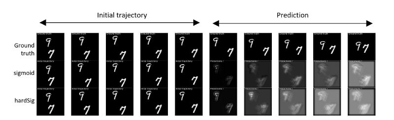Figure 14: The history and predicted frames using logsig and hardSig as gate activations. Except for the ‘double exposure effect,’ the predicted shape is preserved.

Table 3: The Non-Gate Unit Effect on Training.

Activation function		Training Results
	Time	Loss	Val-loss	Mean Absolute	Accuracy	SE
	(Minutes)	(MSE)	(MSE)	Error (MAE)	(Percentage)	(Loss)
sigmoid	24.5	0.00367	0.00387	0.02597	0.93058	0.0000438
tanh	23.9	0.00423	0.00537	0.01751	0.93003	0.0000607
hardSig	25.3	0.00347	0.00386	0.02401	0.93076	0.0000300
softSign	23.9	0.00431	0.00442	0.01777	0.92972	0.0001690
softPlus	24.2	0.00342	0.00308	0.02044	0.93073	0.0000400
ReLU	23.7	0.00424	0.00451	0.01911	0.93015	0.0000723
ELU	23.6	0.00453	0.00555	0.01760	0.93001	0.0001431
SELU	26.5	0.00392	0.00407	0.01784	0.93031	0.0001984

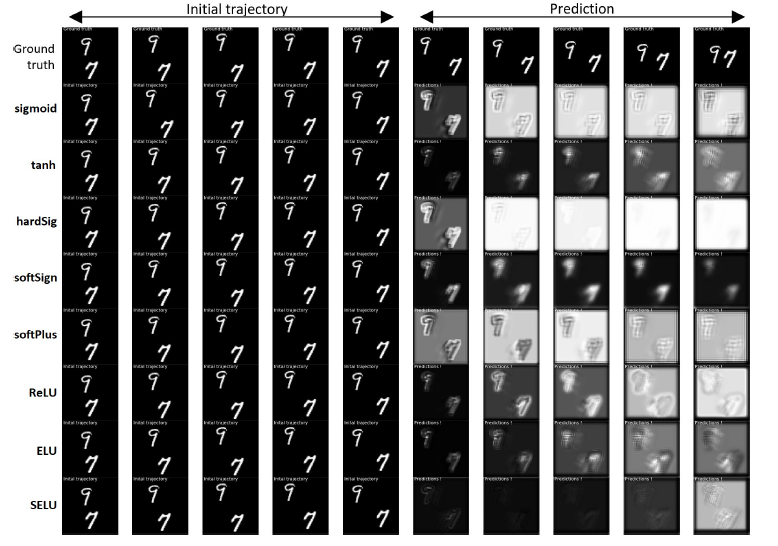Figure 15: The initial trajectory and predicted frames for each non-gate unit activation function. Although there is shape distortion, the movement directions seem to be preserved.

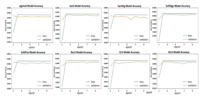Figure 16: Training and validation accuracy non-gate unit activations. All tested functions are shown for each training epoch.

always set to hardSig. This happens to be the default recurrent activation in the Keras convLSTM API.

There is no restriction on the range of the unit activation function selection compared to the gate activation. Therefore, we tested all eight of the functions from Section 3. Table 3 shows average training time, training loss, validation loss, validation mean absolute error, training accuracy, and standard error of training loss (n = 3). The units of training and validation loss are MSE.

Table 3 shows that the elapsed training time of the functions is overall about the same and the highest training time (SELU) is about two minutes longer than the rest. Loss was calculated using MSE and is about the same for all tested functions.

Accuracy of the training and validation tests appears in Figure 16 where the hardSig has the lowest validation accuracy because the accuracy degraded over time. In addition, it has a significant average difference between both the training and validation accuracy curves. For the SoftPlus, SELU, ReLU, and ELU diagrams, there is a notable unstable validation accuracy compared to the training accuracy. However, the most stable validation accuracy for the other tested functions is found when the activation was sigmoid, tanh, or the softSign function. However, the average difference between training and validation accuracies for logsig is higher than the tanh and softSign.

The predicted videos as compared with ground truth for the non-gate unit functions is shown in Figure 15. The lowest visual accuracy occurs when the SELU function is used. The hardSig, logsig, ReLU, and softPlus functions show roughly the same visual prediction results. These functions were unable to maintain, the object’s outline, the background, or object’s color. The ELU function could not retain the digit outline through time. The softSign function was able to maintain the shape of the objects but it maintained the object’s location with reducing their actual sizes. It also suppressed object movement. The tanh preserved the object shape and movement.

In important insight can be seen by looking at the differential visual prediction results in Figure 15. Although changing the non-gate activation functions changes the shape distortion, the predicted movement accuracy seems to be the same across the different activation functions. This indicates that non-gate units play more of a role in predicted shape than in predicting movement direction. In contrast, we saw the opposite pattern with the gate activation functions.

As seen in Figures 14 and 15, prediction accuracy should be improved for practical applications. The intent of our work was to study differential activation function effects. Prediction accuracy can be improved by enhancing the model architecture by increasing the number of the convolutional LSTM layers and adding regularization techniques such as dropout [35]. Further improvements can be obtained by adding more channels to each layer, increasing the number of training epochs, adjusting the input batch size, and adjusting the hyper-parameters. Moreover, using an information flow propagation transfer algorithm (such as predictive coding [4, 36, 37]) to data between the multilayered hierarchy could significantly increase the prediction performance.

5. Conclusion

We found that the choice of gate unit activation function, when used in the convLSTM video prediction problem, affects acquisition of the digit’s movement trajectory throughout the video frame sequence. The role of the non-gate unit activation is to enhance the object’s shape and determine its details. Only activation functions with range [0,1] are eligible as a gate activation functions. The convLSTM exhibited the best prediction performance when the gate activation used the hardSig function and it had the best prediction visual results. In addition, the relation between training and validation accuracies was stable. The model also obtained better predictions when the tanh function was used as the non-gate activation. The tanh has similar training loss and training time to the other functions examined in our experiments.

1.  M. Baccouche, F. Mamalet, C. Wolf, C. Garcia, and A. Baskurt, “Sequential deep learning for human action recognition,” in InternationalWorkshop on Human Behavior Understanding, pp. 29–39, Springer, 2011.
2.  T. Pham, T. Tran, D. Phung, and S. Venkatesh, “Deepcare: A deep dynamic memory model for predictive medicine,” in Pacific-Asia Conference on Knowledge Discovery and Data Mining, pp. 30–41, Springer, 2016.
3.  X. Shi, Z. Chen, H. Wang, D.-Y. Yeung, W.-K. Wong, and W.- c. Woo, “Convolutional LSTM network: A machine learning approach for precipitation nowcasting,” in Advances in neural information processing systems, pp. 802–810, 2015.
4.  W. Lotter, G. Kreiman, and D. Cox, “Deep predictive coding networks for video prediction and unsupervised learning,” arXiv preprint arXiv:1605.08104, 2016.
5.  N. Elsayed, A. S. Maida, and M. Bayoumi, “Reduced-gate convolutional LSTM using predictive coding for spatiotemporal prediction,” arXiv preprint arXiv:1810.07251, 2018.
6.  L. Medsker and L. Jain, “Recurrent neural networks,” Design and Applications, vol. 5, 2001.
7.  S. Hochreiter and J. Schmidhuber, “Long short-term memory,” Neural computation, vol. 9, no. 8, pp. 1735–1780, 1997.
8.  F. A. Gers, J. Schmidhuber, and F. Cummins, “Learning to forget: Continual prediction with LSTM,” Neural Computation, 2000.
9.  I. Goodfellow, Y. Bengio, and A. Courville, Deep Learning. MIT Press, 2016. http://www.deeplearningbook.org.
10.  F. A. Gers, N. N. Schraudolph, and J. Schmidhuber, “Learning precise timing with LSTM recurrent networks,” Journal of machine learning research, vol. 3, no. Aug, pp. 115–143, 2002.
11.  G.-B. Zhou, J. Wu, C.-L. Zhang, and Z.-H. Zhou, “Minimal gated unit for recurrent neural networks,” International Journal of Automation and Computing, vol. 13, no. 3, pp. 226–234, 2016.
12.  K. Greff, R. K. Srivastava, J. Koutnik, B. R. Steunebrink, and J. Schmidhuber, “LSTM: A search space odyssey,” IEEE Transactions on Neural Networks and Learning Systems, vol. 28, pp. 2222– 2232, Oct 2017.
13.  N. Kalchbrenner, A. v. d. Oord, K. Simonyan, I. Danihelka, O. Vinyals, A. Graves, and K. Kavukcuoglu, “Video pixel networks,” arXiv preprint arXiv:1610.00527, 2016.
14.  C. Finn, I. Goodfellow, and S. Levine, “Unsupervised learning for physical interaction through video prediction,” in Advances in neural information processing systems, pp. 64–72, 2016.
15.  Y. Wang, M. Long, J. Wang, Z. Gao, and S. Y. Philip, “PredRNN: Recurrent neural networks for predictive learning using spatiotemporal LSTMs,” in Advances in Neural Information Processing Systems, pp. 879–888, 2017.
16.  K. T. P. D. L. library, “Keras documentation,” 2018.
17.  N. Srivastava, E. Mansimov, and R. Salakhudinov, “Unsupervised learning of video representations using LSTMs,” in International conference on machine learning, pp. 843–852, 2015.
18.  N. Elsayed, A. S. Maida, and M. Bayoumi, “Empirical activation function effects on unsupervised convolutional LSTM learning,” in 2018 IEEE 30th International Conference on Tools with Artificial Intelligence (ICTAI), pp. 336–343, IEEE, 2018.
19.  A. Graves, N. Jaitly, and A.-r. Mohamed, “Hybrid speech recognition with deep bidirectional LSTM,” in Automatic Speech Recognition and Understanding (ASRU), 2013 IEEE Workshop on, pp. 273–278, IEEE, 2013.
20.  A. Graves and N. Jaitly, “Towards end-to-end speech recognition with recurrent neural networks,” in International Conference on Machine Learning, pp. 1764–1772, 2014.
21.  M. Sundermeyer, R. Schl¨uter, and H. Ney, “LSTM neural networks for language modeling,” in Thirteenth annual conference of the international speech communication association, 2012.
22.  S. Ruder, P. Ghaffari, and J. G. Breslin, “A hierarchical model of reviews for aspect-based sentiment analysis,” arXiv preprint arXiv:1609.02745, 2016.
23.  D. Eck and J. Schmidhuber, “A first look at music composition using LSTM recurrent neural networks,” Istituto Dalle Molle Di Studi Sull Intelligenza Artificiale, vol. 103, 2002.
24.  F. Ord´o˜nez and D. Roggen, “Deep convolutional and LSTM recurrent neural networks for multimodal wearable activity recognition,” Sensors, vol. 16, no. 1, p. 115, 2016.
25.  O. Vinyals, A. Toshev, S. Bengio, and D. Erhan, “Show and tell: A neural image caption generator,” in Proceedings of the IEEE conference on computer vision and pattern recognition, pp. 3156– 3164, 2015.
26.  S. Bengio, O. Vinyals, N. Jaitly, and N. Shazeer, “Scheduled sampling for sequence prediction with recurrent neural networks,” in Advances in Neural Information Processing Systems,pp. 1171–1179, 2015.
27.  M. Schtickzelle, “Pierre-Franc¸ois Verhulst (1804-1849). La premi`ere d´ecouverte de la fonction logistique,” Population (French edition), pp. 541–556, 1981.
28.  C. Gulcehre, M. Moczulski, M. Denil, and Y. Bengio, “Noisy activation functions,” in International Conference on Machine Learning, pp. 3059–3068, 2016.
29.  J. Bergstra, G. Desjardins, P. Lamblin, and Y. Bengio, “Quadratic polynomials learn better image features,” Technical report, 1337, 2009.
30.  Y. W. Teh and G. E. Hinton, “Rate-coded restricted Boltzmann machines for face recognition,” in Advances in neural information processing systems, pp. 908–914, 2001.
31.  C. Dugas, Y. Bengio, F. B´elisle, C. Nadeau, and R. Garcia, “Incorporating second-order functional knowledge for better option pricing,” in Advances in neural information processing systems, pp. 472–478, 2001.
32.  D.-A. Clevert, T. Unterthiner, and S. Hochreiter, “Fast and accurate deep network learning by exponential linear units (ELUS),” arXiv preprint arXiv:1511.07289, 2015.
33.  D. P. Kingma and J. Ba, “Adam: A method for stochastic optimization,” arXiv preprint arXiv:1412.6980, 2014.
34.  Z. Wang and A. C. Bovik, “A universal image quality index,” IEEE signal processing letters, vol. 9, no. 3, pp. 81–84, 2002.
35.  N. Srivastava, G. Hinton, A. Krizhevsky, I. Sutskever, and R. Salakhutdinov, “Dropout: a simple way to prevent neural networks from overfitting,” The Journal of Machine Learning Research, vol. 15, no. 1, pp. 1929–1958, 2014.
36.  J. M. Kilner, K. J. Friston, and C. D. Frith, “Predictive coding: an account of the mirror neuron system,” Cognitive processing, vol. 8, no. 3, pp. 159–166, 2007.
37.  R. P. Rao and D. H. Ballard, “Predictive coding in the visual cortex: a functional interpretation of some extra-classical receptive-field effects,” Nature neuroscience, vol. 2, no. 1, p. 79, 1999.

(Click Here)

(Click Here)