1. Introduction

Dynamical equation models, which comprise of the linear, complex, and hybrid dynamical system, play an important role in engineering the control systems. There are thousands of published research articles developed to analyze the dynamical model of some new engineering systems such as the mobile robot [1, 2], autonomous vehicles, car-like robot, etc. This research deals with an independent system with some known initial state and its corresponding output value with plant’s initial position. The plant utilized moves to a decided state known as target position with minimal “effort” where some restricted states are not allowed to be passed through by the plant. The term “effort” in some cases is defined as the shortest path, while an obstacle is a restriction in space movement which should be avoided by the plant. The pioneer mathematical model utilized in this state was developed in [3] by formulating a piecewise affine model which corresponds to the restricted and normal sets. There are some published articles which described the restricted use of some systems, such as vehicles and mobile robots [4–9]. The more complicated problem comprises of several plants which are controlled by applying a multi-agent concept like flocking scheme, which was used in [10,11].

In some cases, the objectives of restricted area avoidance are not only avoiding the obstacle but also determining the optimal trajectory used to determine the final or target point. In this problem, an optimal control method based on mathematical optimization was implemented to solve the technique. For example, a particle swarm algorithm was applied in [12,13]. It is reasonable to utilize an optimization-based method because it will generate the ace result to the problem. Beside of optimal control problem, numerous inconsistencies were solved using the optimization approach which was also used to describe its profitability such as facility location optimization and the colony algorithm for knapsack.

In the system theory, a newly developed strategy is the hybrid dynamical model which comprises of different types of Piecewise-affine (PWA), discrete hybrid automata (DHA) and Mixed Logical Dynamic (MLD) models [14]. To analyze and control a hybrid model, in [15], a toolbox was developed which comprises of some MATLAB functions on model formulation and controlling. For example, the PWA model written in HYSDEL programming language can be converted into MLD using the MATLAB routine “mld” in the hybrid system toolbox. Furthermore, the MLD model which consists of trajectory tracking problems tends to be solved by applying a classic control method scheme MPC (model predictive control) and modifying the state prediction along with its corresponding objective function which was carried out in [16,17]. Many research articles applied this control method in agriculture field [18,19], as well as in controlling mechanical vehicles [20], boiler-turbine [21], and spacecrafts [22].

This research therefore aims at solving the problem associated with the restricted area inherent the three-dimensional states. First, the PWA model was formulated to determine whether the dynamical system of the plant is in a normal or restricted area. Next, the PWA system is converted into equivalent MLD using HYSDEL and hybrid toolbox. Furthermore, by using predictive control method for the MLD model, the optimal input was generated to obtain the moving trajectory, which was initialized at the plant’s starting point to its target position. Some computational simulations are performed to illustrate and visualize the results.

2. Dynamical System

Let vector denotes the state of a plant where k denotes the time instantly. Therefore, the dynamical model of the observed plant is a linear time-invariant system modeled as illustrated in the equation below

where  and  are input & output vectors respectively, and the notations A, B, C, and D are real constant matrices. The control method used in this paper is applicable, the controllable and observable assumptions are held by .

2.1.  Restricted Area Avoidance Scheme

The position to the output vector y is defined without losing the generality property. Let the initial position of the plant is obtained by . The value of the output, i.e., plant’s position y have to maneuver and reach some desired target position denoted by  which corresponds to target state , , where in the output’s domain, some sets such as  are not allowed to be utilized by y. Let , y is restricted to be in R, then  should be held. To handle this condition, the dynamics of the system is formulated as a hybrid system.

The formula is illustrated as follows, w.l.o.g., let  with two restricted sets, R₁ and R₂ illustrated in Figure 1. The problem is how to determine the optimal trajectory used by the plant to maneuver (or move) from its initial state to the target position. The term “optimal” is interpreted as minimal effort (or energy or work or other similar things) used by the plant. The optimal trajectory shown in Figure 1 illustrates a moving trajectory from the initial to the target point.

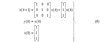
 The non-restricted sets are known as the normal area where the dynamics of the plant corresponds to . Alternatively, the dynamics which corresponds to the restricted set is defined as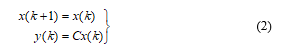

which means that the dynamical model is used to prevent the plant from being located in the restricted area.  The formulation of the hybrid dynamical model where the plant is prevented from entering the restricted area is illustrated by Figure 2 by assuming  and .

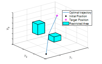Figure 1: Two box-shape restricted areas illustration

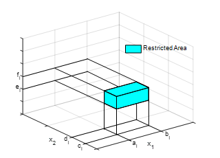Figure 2: Restricted area labeling

Let the restricted sets (area) R_i, i = 1, 2, …, k, and the normal set (area) denoted by N, then these sets are written as

2.2.  PWA to MLD Hybrid Model

The hybrid model in the PWA model of the plant for restricted area avoidance purposes is formulated as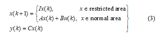

with I denotes an identity matrix with the appropriate dimension. To apply the predictive control method to this system, the MLD model is, first of all, converted into the form of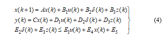

with some initial state where  is an auxiliary state. The notation  is a binary valued state describing the mode of the system (mode 0 assuming it is on the normal area and 1 when restricted). The matrices  and  for all i are real constant generated by the conversion process, which is conducted using mld MATLAB function embedded in hybrid system toolbox given in [23] by writing the PWA system in HYSDEL, then generating the matrices for the equivalent MLD model.

2.3.  Predictive Control Approach

The equation used to determine the optimal input to enable the output vector (position) reach the target point using minimal effort is represented as a terminal state optimal control problem. Furthermore, the predictive control approach is used to obtain the optimal input by letting  as the state value predicted at time instant  which is resulted by applying input value  into equation where the corresponding output value is predicted at time instant , . The optimal input will be calculated by solving the minimal value “cost” function of output prediction as follows: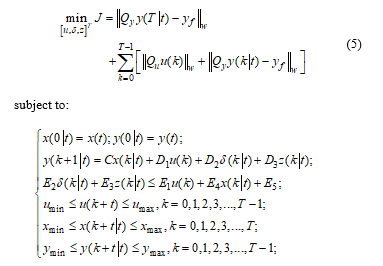

where T is called the horizon control period, Q_u and Q_y are symmetric and positive definite matrices used to weight the input u and output y respectively. These symmetric and positive definite properties are applied to guarantee the objective function J is convex. This is expressed in the notation  where . This predictive control scheme resulting in a mixed integer quadratic optimization problem and in our simulation, miqp MATLAB function, which is also embedded in hybrid system toolbox, is utilized to solve. Finally, the optimal values of u(k) for all k are used by the system. For restricted area purposes, the term y_f in is the final/target position where the dynamics of x is (4) which equivalents to .

3. Simulation Results

Given a plant with three-dimensional state and output vector  which can be described as the position in a three-dimensional Cartesian coordinate system. Let the initial state be , which corresponds to the initial position .

SYSTEM pwa_obs_3d_robot {

INTERFACE { STATE { REAL x1 [-20,20];

                    REAL x2 [-20,20];

                    REAL x3 [-20,20]; }

    INPUT { REAL u [-10,10]; }

            OUTPUT{ REAL y1,y2,y3; }

            PARAMETER { REAL a1;        REAL a2;

        REAL b1;        REAL b2;

        REAL c1;        REAL c2;

        REAL d1;        REAL d2;

                REAL e1;        REAL e2;

                        REAL f1;         REAL f2; } }

IMPLEMENTATION { AUX { REAL z1,z2,z3;

                 BOOL da1,da2,db1,db2,dc1,dc2,

      dd1,dd2,de1,de2,df1,df2; }

                 AD  {da1 = x1>=a1;      da2 = x1>=a2;

              db1 = x1>=b1;      db2 = x1>=b2;

                      dc1 = x2>=c1;      dc2 = x2>=c2;

                      dd1 = x2>=d1;      d2 = x2>=d2;

                      de1 = x3>=e1;      de2 = x3>=e2;

                      df1 = x3>=f1;      df2 = x3>=f2; }

DA  {z1 = {IF

    (da1&~db1)&(dc1&~dd1)&(de1&~df1)

    THEN x1 ELSE x1+u }; z2 = {IF

    (da2&~db2)&(dc2&~dd2)&(de2&~df2)

       THEN x2 ELSE x2+u }; z3 = {IF

    (da3&~db3)&(dc3&~dd3)&(de3&~df3)

    THEN x3 ELSE x3+u }; }

                    CONTINUOUS {x1 = z1;

                                x2 = z2;

                                x3 = z3; }

                    OUTPUT { y1 = x1;

                             y2 = x2;

                             y3 = x3; } } }

Listing Code 1: PWA model with two restricted areas in HYSDEL

Then the dynamic of the plant in the normal area is Suppose there are two restricted sets R₁ and R₂ defined visually as two boxes

where the rest of state space is normal, then the PWA model of this system is stated as

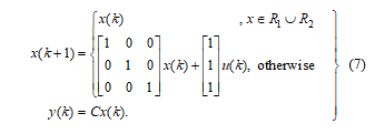
The PWA model in HYSDEL has already been written (See Listing Code 1) and converted it into MLD model resulting in the following matrices and E₁, E₂, E₃, E₄, and E₅ because their dimension is sufficiently large.

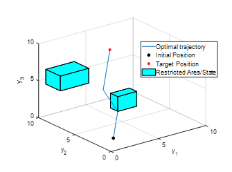Figure 3: Optimal moving trajectory generated by the controller

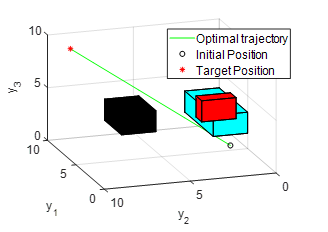Figure 4: Optimal moving trajectory with three box-shape restricted area

By solving with w=2, the optimal input values are obtained, and by applying them into , the optimal moving trajectory from its initial position to its target/final position as show in Figure 3 of the output values are obtained. From Figure 3, it is observed that two restricted areas were restricted and avoided by the system’s moving trajectory, as illustrated in the two boxes. For further simulation, another box was added. The result is shown in Figure 4 and is similar to the optimal moving trajectory, which was generated by the controller to prevent the restricted areas.

4. Conclusions

The multi-restricted area which avoids the problem associated with the autonomous linear system was considered dynamic with the region formulated as a hybrid model and the optimal trajectory calculated. From the computational simulation, the obtained system’s moving trajectory was generated by the controller, and the given restricted areas were avoided. Further research works will develop the shape of the restricted area into other shapes like polytope to control the inconsistencies associated with irregular shapes. Other control methods will be considered and compared to determine the best in performance.

Conflict of Interest

The authors declare no conflict of interest regarding this work.

Acknowledgment

This work was funded by Universitas Diponegoro under RPI 2019 research grant.

1.  E. S. Briskin, Y. V. Kalinin, A. V. Maloletov, and N. G. Sharonov, “Mathematical Modelling of Mobile Robot Motion with Propulsion Device of Discrete Interacting with the Support Surface,” IFAC-PapersOnLine, 51(2), 236–241, 2018. https://doi.org/10.1016/j.ifacol.2018.03.041
2.  Y. L. Kuo, “Mathematical modeling and analysis of the Delta robot with flexible links,” Comput. Math. with Appl., 71(10), 1973–1989, 2016. http://dx.doi.org/10.1016/j.camwa.2016.03.018
3. J. J. A. M. Keij, “Obstacle Avoidance with Model Predictive Control in a Hybrid Controller,” (technical report), 2002.
4.  Sutrisno, Salmah, E. Joelianto, A. Budiyono, I. E. Wijayanti, and N. Y. Megawati, “”Model Predictive Control for Obstacle Avoidance as Hybrid Systems of Small Scale Helicopter,” in 3rd International Conference on Instrumentation Control and Automation (ICA), 2013, pp. 127–132. DOI: 10.1109/ICA.2013.6734058
5.  Z. Yan, Y. Zhao, S. Hou, H. Zhang, and Y. Zheng, “Obstacle Avoidance for Unmanned Undersea Vehicle in Unknown Unstructured Environment,” Mathematical Problems in Engineering, 2013, 1-12, 2013. http://dx.doi.org/10.1155/2013/841376
6.  R. Wang, M. Wang, Y. Guan, and X. Li, “Modeling and Analysis of the Obstacle-Avoidance Strategies for a Mobile Robot in a Dynamic Environment,” Mathematical Problems in Engineering, 2015, 1-11, 2005. http://dx.doi.org/10.1155/2015/837259
7.  D. Q. Bao and I. Zelinka, “Obstacle Avoidance for Swarm Robot Based on Self-Organizing Migrating Algorithm,” Procedia Comput. Sci.,150, 425–432, 2019. DOI: 10.1016/j.procs.2019.02.073
8.  Y. Zhao, X. Chai, F. Gao, and C. Qi, “Obstacle avoidance and motion planning scheme for a hexapod robot Octopus-III,” Rob. Auton. Syst., 103, 199–212, 2018. DOI: 10.1016/j.robot.2018.01.007
9.  Y. Gao, Y. Wu, X. Yang, C. Liao, K. Cheng, and H. Luo, “Reactive obstacle avoidance of monocular quadrotors with online adapted depth prediction network,” Neurocomputing, 325, 142–158, 2018. https://doi.org/10.1016/j.neucom.2018.10.019
10.  J. Wang et al., “An Improved Fast Flocking Algorithm with Obstacle Avoidance for Multiagent Dynamic Systems,” Journal of Applied Mathematics, 2014, 1-13, 2014. http://dx.doi.org/10.1155/2014/659805
11.  Z. Chen, L. Ding, K. Chen, and R. Li, “The Study of Cooperative Obstacle Avoidance Method for MWSN Based on Flocking Control,” The Scientific World Journal, 2014, 1-12, 2014. http://dx.doi.org/10.1155/2014/614346
12.  T. Yang, Z. Liu, H. Chen, and R. Pei, “Robust Tracking Control of Mobile Robot Formation with Obstacle Avoidance,” Journal of Control Science and Engineering, 2007, 1-10, 2007. http://dx.doi.org/10.1155/2007/51841
13.  G. S. Chyan and S. G. Ponnambalam, “Robotics and Computer-Integrated Manufacturing Obstacle avoidance control of redundant robots using variants of particle swarm optimization,” Robot. Comput. Integr. Manuf., 28(2), 147–153, 2012. DOI: 10.1016/j.rcim.2011.08.001
14. A. Bemporad, “Efficient conversion of mixed logical dynamical systems into an equivalent piecewise affine form,” IEEE Trans. Automat. Contr., 49(5), 832–838, 2004. DOI: 10.1109/TAC.2004.828315
15.  A. Bemporad, “Hybrid Toolbox User’s Guide,” Lucca, 2012.
16.  F. Borrelli, A. Bemporad, and M. Morari, Predictive Control for linear and hybrid systems. Cambridge, UK: Cambridge University Press, 2014.
17.  J. M. Maciejowski, Predictive Control with Constrains. USA: Prentice Hall, 2001.
18.  Y. Ding, L. Wang, Y. Li, and D. Li, “Model predictive control and its application in agriculture: A review,” Comput. Electron. Agric., 151, 104–117, 2018. https://doi.org/10.1016/j.compag.2018.06.004
19.  L. Chen, S. Du, Y. He, M. Liang, and D. Xu, “Robust model predictive control for greenhouse temperature based on particle swarm optimization,” Inf. Process. Agric., 5(3), 329–338, 2018. https://doi.org/10.1016/j.inpa.2018.04.003
20.  M. Jalali, E. Hashemi, A. Khajepour, S. Chen, and B. Litkouhi, “Model predictive control of vehicle roll-over with experimental verification,” Control Eng. Pract., 77, 95–108, 2018. DOI: 10.1016/j.conengprac.2018.04.008
21.  X. Liu and J. Cui, “Economic model predictive control of boiler-turbine system,” J. Process Control, 66, 59–67, 2018. https://doi.org/10.1016/j.jprocont.2018.02.010
22.  P. Li and Z. H. Zhu, “Model predictive control for spacecraft rendezvous in elliptical orbit,” Acta Astronaut., 146, 339–348, 2018. https://doi.org/10.1016/j.actaastro.2018.03.025
23. F. D. Torrisi and A. Bemporad, “HYSDEL — A Tool for Generating Computational Hybrid Models for Analysis and Synthesis Problems,” IEEE Trans. Control Syst. Technol., 12(2), 235–249, 2004. DOI: 10.1109/TCST.2004.824309

(Click Here)

(Click Here)