1. Introduction

Environmental sound recognition (AESR) is a relatively new discipline of computer science destined to extend the field of speech-based applications, or the study of music sounds, by exploring the vast range of environmental non-speech sounds.

This paper is an extension of work originally presented in the 43^rd International Conference on Telecommunications and Signal Processing, held in Milan in July 2020 [1]. It investigates several sound modelling and classification paradigms, in the context of a forest monitoring system.

The new research area of AESR is intended to simulate the important function of human hearing, and possibly, to overpower human perception. This is motivated by the fact that hearing is the human second most important sense after vision and should not be disregarded when trying to build a computer that simulates human behaviour and senses. Consequently, AESR recently became an essential field of computer science [2]-[4].

By environmental sounds we mean everyday sounds, natural or artificial, other than speech. Natural sounds may be leaves rustling, animal noise, birds chirping, water ripple, wind blowing through trees, waves crashing onto the shore, thunder. Artificial sounds include sounds produced by diverse engines like cars, cranes, ATVs, snowmobile, lawnmower, pneumatic hammer, chainsaw, etc., but also creaky doors or creaky floors, gunshots, crowd in a club, breaking glass, vehicle tyres or brake noise. The environments where this discipline is applied are also very diverse, falling into two broad categories:

• Natural environment like forest environment, ecological units, seashore environment; however, the degree of naturalness is variable, and purely natural environments are very rare as one may intercept voices, vehicle sounds, chainsaw in forests or even jungle.
• Built environment, also called human made environment, like the urban environment, the household, maybe agricultural environment, harbours; obviously in any of these environments, natural acoustic events, like thunder, rain falling, wind blowing may also happen.

In reality there are no purely natural or artificial sounds, neither purely speech nor non-speech acoustic events. Most of the application investigate mixed environments where natural and artificial, speech or non-speech acoustic events are equally possible.

The applicability of AESR is related to the advent of Internet of Things (IoT). IoT devices have sensors, possibly acoustic, and software that enable the collection and exchange of data through the Internet. Automatic recognition of the surrounding environment allows devices to switch between tasks with minimum user interference [5]. For a robot, audio recordings may provide important information about location and direction of a moving vehicle, or environmental information, such as speed of wind.

AESR has an important role in security, environment protection or environment research. Among possible applications are the identification of deforestation threats and illegal logging activities, through automatic detection of specific sounds like several engines, chainsaws, or vehicles. Detecting other illegal activities like hunting in forest or ecological reserves, by spotting gun shots, or human voices would be a useful application [6]-[9]. In recent times, solutions based on environmental sound recognition are applied in early wildfire detection [10].

Another type of applications concerns scientific monitoring of the environment. Such applications are intended for instance, to detect species, by discrimination between different animals or birds’ sounds [11], [12].

Computational Auditory Scene Analysis (CASA), is a very complex field of AESR, aimed to the recognition mixtures of sound sources by simulating human listening perception using computational means. It mainly addresses two important tasks, Environmental Audio Scene Recognition (EASR) and Sound Event Recognition (SER) and has a huge importance in environment audio observation and surveillance. EASR refers to recognition of indoor or outdoor acoustic scenes (e.g., cafes/restaurants, home, vehicle or metro stations, supermarkets, versus crowded or silent streets, forest landscape, countryside, beaches, gym halls, swimming pools). SER is intended to the investigation of specific acoustic events in the audio environments, like dog barking, gunshots, sudden brake sounds, or human non-speech events, like coughing, whistling, screaming, child crying, snoring, sneezing [13].

An emerging field is the investigation and detection of acoustic emissions, used in monitoring landslide phenomena [14]. Acoustic emissions (AE) are elastic waves generated by movement at particle-to-particle contacts and between soil particles and structural elements. They are not perceived by the human ear, are super audible, and therefore their frequencies are very high, expected to range between 15kHz and 40 kHz. The devices used to acquire these waves should ensure a sampling frequency of over 80 kHz. AE monitoring is an active area, not very well developed due to low energy levels of these waves, which make it challenging to detect and quantify [15], [16].

Likewise, recent studies have shown that moving avalanches emit a detectable sub-audible sound signature in the low frequency infrasonic spectrum [17].

The study of underwater acoustic infrasonic emissions, provided by hydrophones, is another field of AESR research [18].

Our paper explores forest acoustics aiming to find the suitable sound modelling and classification approaches. The focus of our research is the detection of logging risk by identification of specific classes of sounds: chainsaw, vehicles, or possibly speech. We extend an earlier research on acoustic signal processing, by exploring the dominant paradigm in data modelling and, the deep neural networks (DNN). We investigate two types of DNNs, the Deep Feed Forward Neural Networks (FFNN) and a popular version of Recurrent Neural Networks (RNNs), the Long Short-Term Memory (LSTM).  The two neural networks will be run on two types of feature spaces: the Mel-cepstral and the Fourier log-power spectrum feature spaces. We will compare their results with the former performance obtained using the Gaussian Mixtures Modelling (GMM) and the Dynamic Time Warping (DTW) in the context of a closed-set identification system. One main goal is to stress the importance of feeding as input to DNN less processed features, like log-power spectrum, as compared to the more elaborate sets of features, e.g., Mel-frequency cepstral features.  Another purpose of the paper is to clarify some issues concerning signal pre-processing framework, like length of the analysis window and the underlying frequency domain to be used in spectral analysis.

The paper is structured as follows: the next section describes the state-of-the-art in environmental sound recognition; the third section details our approach, the signal feature extraction and modelling methods we applied in sound recognition; the fourth section presents the setup of the experiments and evaluates the proposed methods; the last part presents the conclusions of the paper.

2. State-of-the-art

Early attempts [2], [19] to assess speech typical methods in the context of non-speech acoustics, analyse classical methods like Artificial Neural Networks (ANN), or Learning Vector Quantization (LVQ), on Fourier, or Linear Predictive Coding (LPC) feature spaces.

In [20], the authors make an overall investigation of recognition methodologies for different categories of sounds. The environmental sounds are classified as stationary and non-stationary. The framework used for stationary acoustic signals coincides to a great extent with the one used in voice-based applications (speech or speaker recognition) in what concerns the specific features and feature space modelling methods. For feature extraction, the spectral features, like those derived from Mel analysis – Mel Frequency Cepstral Coefficients (MFCCs), LPC, Code Excited Linear Prediction (CELP), or techniques based on signal autocorrelation, prevail. The modelling approaches are also shared with voice-based applications: GMM, k-Nearest Neighbours (k-NN), Learning Vector Quantisation (LVQ), DTW, Hidden Markov Models (HMM), Support Vector Machine (SVM), Neural Networks, and deep learning. Concerning non-stationary signals, some successful techniques are based on sparse representations like the Matching Pursuit (MP) and MP-Gabor features. Alternative approaches use fusion of MFCC and other parameters to boost the performance.

In [5], the authors review the current methodologies used in AESR and evaluate their performance, efficiency, and computational cost. The leading approaches of the moment are GMM, SVM and DNN or Recurrent Neural Networks (RNN) The paper describes open-set identification experiments on two types of acoustic events, baby cries and smoke alarm, and a very large range of complementary environment acoustic events. as impostor data. In this respect GMM, using the Universal Background Model (GMM-UBM) and two neural network architectures were compared. The Deep Feed Forward Neural Network yielded the best identification rate, while the best computational cost is made by GMM. SVM has an intermediate identification rate, yet at a high computational cost, assessed accounting for four basic operations: addition, comparison, multiplication, and lookup table retrieval (LUT). The computational cost is a critical feature in the context of IoT, where sound analysis applications are required to run on embedded platforms with hard constraints on the available computing power.

In [13], the authors make a thorough and extensive investigation of the most recent achievements and tendencies in AESR, more precisely in EASR and SER fields of CASA. from the perspective of acoustic feature extraction, the modelling methodology, performance, available acoustic databases. Besides the conventional approaches, new classes of features were applied lately by several implementations. Such characteristics are the auditory image-based features, basically regarding the time-frequency spectrograms as bidimensional images. where the frequency is not necessarily in the linear domain, but possibly adapted to a perceptual scale. Besides the log-power spectrum, Mel or Bark-frequency log-scale spectrograms, Spectrogram Image Features (SIF) [21], such characteristics as Mel scale with Constant-Q-Transform [22], wavelet coefficients [23] are referred.

Another class of features are generated by learning approaches with the goal to provide lower and enhanced representations. Such features are obtained applying techniques like quantization, i-vector, non-negative matrix factorization (NMF) [24], sparse coding, Convolutional Neural Network–Label Tree Embeddings (CNN-LTE) [25], etc.

Concerning the experimented methodologies, the deep learning methods are predominant, with Feed-Forward Neural Networks and Convolutional Neural Networks (CNN) in the leading position.  Many strategies are currently operating CNNs in conjunction with a variety of features, among which log-scaled mel-spectrograms [26]-[28], CNN-LTE [25] or in hybrid approaches [29]. These implementations outperformed the other attempts to approach EASR and SER tasks.

Avalanche or landslide monitoring applications use methodologies based on thresholds for acoustic emissions energy, depending on the hazard risk level.

Concerning the general framework applied in AESR, we draw on the ideas presented in [20]. The usual pre-processing of the acoustic signal, applied in AESR includes a framing step, possibly followed by sub-framing or sequential processing. In the “framing” stage the signal is processed continuously, frame by frame. A classification decision is made for each frame and successive frames may belong to different classes. This is illustrated in figure 1, where a chainsaw is detected in a forest environment. Framing can enhance the acoustic signal classification by structuring the stream into more homogeneous blocks to better catch the acoustic event. Yet, there is no way of setting an optimal frame length, as for stationary events a length of 3s is a reasonable choice, while for acoustic events like thunder or gunshots, a 3s window length might be too large, and contain other acoustic events, so they could be associated to inappropriate classes. Due to the latest advances in instrumentation, different frame lengths are used to streamline energy consumption during a monitoring process, based on detecting energy levels of environmental sounds.

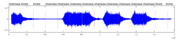Figure 1: Framing process of a real-life sound and classification of each frame

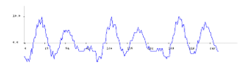Figure 2: 22ms of male speech

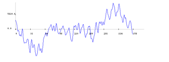Figure 3: 22ms of chainsaw sound

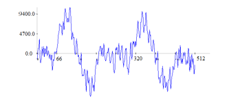Figure 4: 44ms of chainsaw sound

Next, a sub-framing process is applied, by dividing the frame into usually overlapping, analysis subframes. The length of a subframe is explicitly set in [20] to 20-30ms. This length is suited for speech analysis, as it ensures a good resolution in time and frequency. Figure 2 presents 22ms of male speech which includes three fundamental periods of the respective voice. Whereas figure 4 represents 44ms of chainsaw sound which contains two periods of the chainsaw sound. However, we cannot infer anything about the signal periodicity from the segment of 22ms of chainsaw sound, represented in figure 3. Therefore, considering sub-frames of 44ms is a reasonable choice for chainsaw detection. However, a realistic setup must consider a value convenient to all sounds in the acoustic environment.

The further processing applied on the analysis frames is the same with that applied in speech signal analysis and its final goal is to extract characteristic features. The largely applied features are somehow derived from the Fourier features, and called spectral features. Non-spectral features are, for instance, energy, Zero-Crossing Rate (ZCR), Spectral Flatness (SF), all calculated in time domain. Concerning spectral analysis, the relevant frequency interval for a signal sampling frequency of 44.1 kHz is not the whole frequency domain furnished by the Fourier transform, [0, 22.05] kHz, but a shorter range, as shown in figures 5,6. By setting the appropriate analysis frequency interval, we may improve the performance as accuracy and speed of execution, as another benefit of shortening the frequency interval is the decrease of the number of spectrum samples to be processed.

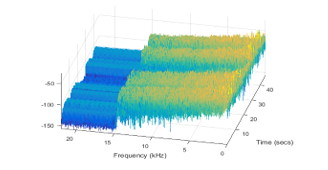Figure 5: Power spectrum of a chainsaw sound

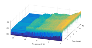Figure 6: Power spectrum of a snowmobile sound

When choosing the spectral analysis, the usual pre-processing on the analysis frame involves (Hamming) windowing and pre-emphasis.

3. The Method

We have applied the framework mentioned above. At framing we divided the audio signal recordings into intervals of 3 seconds. We have used analysis frames of lengths of 22, 44 and 88ms with the usual pre-processing scheme as in speech-based applications. The modelling methods we have evaluated are GMM, DTW and FFNN. As baseline for the feature space, we used the Fourier spectrum coefficients and MFCCs. The set of MFCC parameters was possibly increased with Zero Crossing Rate (ZCR) or/and Spectral Flatness (SF). We have applied GMM on the MFCC feature space, and called this approach MFCC-GMM, DTW on the spectral features space, and FFNN on both the MFCC and spectral features spaces.

3.1. MFCC-GMM

GMM provides probabilistic weighted clustering that generates a coverage of the data space rather than a partition [30], [31]. Each cluster is modelled by a Gaussian distribution, usually called component, defined by the mean m and the standard deviation ? of cluster data, along with a weight w of the component inside the mixture. A data set belonging to the same class C, can be modelled by one or more Gaussian components, and the parameters of each component are calculated using the Estimation-Maximization algorithm, resulting in a model l_C = ((w_k, m_k, ?_k,), k = 1…, K), where K is the number of components. A key step of the algorithm is the initialization where initial values of the parameters (means, variances and weights) are defined. Poor initialization entails bad quality of classification or even impossibility to define the Gaussian parameters. We used at initialization a hierarchical algorithm, Pairwise Nearest Neighbour (PNN) [32] to ensure balanced data clustering, although other hierarchical algorithms such as Complete Linkage Clustering, or Average Linkage Clustering also provide good performance. We have evaluated different distance measures between hierarchy branches: Minkowski (Euclidean distance when square powers are considered), Chebyshev, Euclidian standardised distance. GMM modelling was applied on a feature space consisting of MFCCs and/or Spectral Flatness and ZCR, to generate models for C (C=3) classes of sounds. To classify a sequence of d dimensional features X = {x₁, x₂,…,x_T} into one of the classes its likelihood to belong to each class c is evaluated as

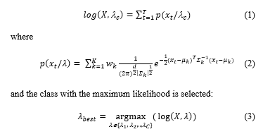Mel frequency analysis [33] [34] is a perceptual approach to signal analysis based on human sensing of the frequency domain. We applied the MATLAB implementations of the Mel-scale frequency:

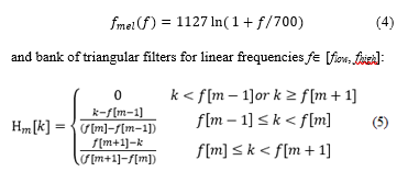The power spectrum calculated on an analysis frame, is passed through the bank filter in (5), and the Mel Frequency Cepstral Coefficients (MFFCs) are derived by applying the Discrete Cosine Transform to the logarithm of the filtered spectrum [33].

Spectral Flatness (tonal coefficient) is meant to highlight noise from tonal sound and is calculated as ratio of geometrical and arithmetical means of spectral coefficients on analysis frames.

A zero crossing arises when two neighbouring samples have opposite signs, and its value on an analysis frame is:3.2. Spectra Alignment using Dynamic Time Warping

Dynamic Time Warping (DTW) measures the similarity of two, usually time-varying, sequences, by optimally aligning them using a recurrent algorithm [35], complying with specific constraints, concerning boundary conditions, monotony, and continuity of the similarity function, and building an optimal path.  One of the issues raised by the DTW algorithm is the long execution time, the main reason for which is the full calculus of DTW matrices, usually defined by distances between the elements of the sequencies. This can be contained by restraining the calculus to a low number of elements, the most likely to participate in the definition of the optimal path by applying an adjusting window as in figure 4, where the popular Sakoe-Chiba band [36] is applied. Figure 7 presents the graphical rendering of a DTW matrix for two sequencies s(t) and r(t), the Sakoe-Chiba band, in grey, highlighting the optimal path, which does not lie entirely inside the band. When applying the Sakoe-Chiba band, the optimal path should lie inside the band and is figured in red in the image, accompanying only inside the band the real optimal path figured in black, thick where it lies within the band.

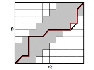Figure 7: Alignment of sequences r, s, using the Sakoe- Chiba band, and the two optimal paths, the real one (black) and the one lying inside the band, which generally coincide.

The DTW algorithm was applied on power spectra of the signal. The power spectrum on an analysis window is calculated as sum of squared Fourier coefficients. One argument for using DTW to align spectral series is the fact that the acoustic signals received from devices of the same type share the same characteristics, such as sampling frequency, so, the generated spectra have the same lengths. Another premise is the fact that the interesting domain for this type of application is under 15 kHz, or even 10 kHz, which is demonstrated by figures 5, 6. This fact is used to align equal length spectra by the DTW algorithm. In the experiments the sampling frequency of the available audio files is equal to 44.1 kHz, the Fourier spectrum covers the domain [0, 22.05] kHz, but if the useful frequency domain is restricted to [0, 7.4] kHz and the analysis frame is of 22ms, the number of features is 171 instead of 512.

Classification of a sequence of feature vectors using the DTW algorithm consists in calculating the distortion between these vectors and the template (training) sequences, and to select the class whose templates show the smallest distortion with respect to the given feature sequence. The calculation involved in this process is based on the distances between individual vectors in the two sets to be compared. The distance may be evaluated in different ways. We have applied two distance measures in the calculus of the distortion measure, the Euclidian norm, and the 1-norm (sum of absolute values).

3.3. Deep feedforward networks (FFNN)

 The artificial neural networks (ANNs) were intended to simulate human associative memory. They learn by processing known input examples, and corresponding expected results, creating weighted associations between them, stored within the network data structure. Deep feedforward networks or multilayer perceptrons (MLPs), are the quintessential deep learning models [37]. The basic unit of a FFNN is the artificial neuron, which expresses the biological concept of neuron [38]. They receive input data, combine the input through internal processing elements like weights and bias terms, and apply an optional threshold using an activation (transfer) function, as shown in figure 8. Transfer functions are applied to provide a smooth, differentiable transition as input values change. They are used to model the output to lie between ‘yes’ and ‘no’, mapping the output values between 0 to 1 or -1 to 1, etc. Transfer function are basically divided into linear and non-linear activation functions. Non-linear transfer functions are “S” – shaped functions like arctg, hyperbolic tangent, logistic functions as in (7):

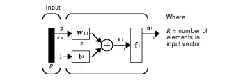Figure 8: Structure of a neuron

The goal of a feedforward network for modelling and classification is to define a mapping  y = f(x,q) and learn the value of parameters θ to ensure the best approximation of the expected value y by the output of f, given the input x and parameters q. FFNNs have one or more hidden layers of sigmoid neurons followed by an output layer of linear neurons. A layer of neurons brings together the weight vectors and biases corresponding to its neurons, so it can be expressed by a matrix of weights and bias vectors, as in figure 9, 10. The transfer function is supposed to be the same for each neuron in the layer. The general diagram of a network is shown in figure 11, where the parameters to be tuned are the weight matrices and bias terms applied at the level of each layer, so that the output of the overall system would be close to expected values. These networks are called feedforward because the information flows in one direction through intermediate computations and there is no feedback connection. The number of neurons does not necessarily decrease with the layer level as presented in figure 10, but usually the goal is to reduce the dimensionality of the input layer, a process similar to feature extraction. The computation corresponding to figure 12 can be expressed by :

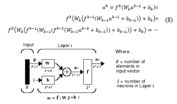Figure 9:  Structure of a layer of neurons

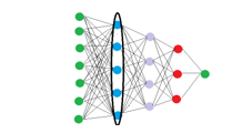Figure 10:  A Feed Forward Neural Network with three highlighted layers

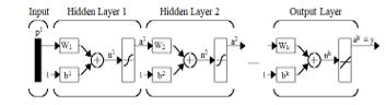Figure 11:   Flow of data in a feedforward network

In equations (8) the known information is

• The input parameters p, which might be measurements from sensors (wind speed, temperature, humidity), parameters coming from images (matrices of colours, or grey hues), or parameters coming from acoustic signals (Fourier spectrum on an analysis window, or more complicated parameters like cepstral, linear prediction coefficients),
• The expected output: for instance, to solve a three classes problem the output corresponding to each class input might be defined as either unidimensional (a scalar value for each class): (-1, 0, 1) or  (0, 1. 2) or multidimensional  (a vector for each class):( (1, 0, 0),  (0, 1, 0),  (0, 0, 1)),
• The neural network architecture: number of hidden layers, number of neurons on each layer, etc.

Unknown parameters are:

• weights at layer k: W_k,
• bias terms at layer k: b_k.

Learning the unknown parameters is performed during the training process. Training of a FFNN can be made in batch mode or in incremental mode [38]. In batch mode, weights and biases are updated after all the inputs and targets are presented. Incremental networks receive the inputs one by one and adapt the weights according to each input. Usually, batch training is used. Equations (8) have as unknowns, the weight matrices and the bias terms, and a much more numerous training known data (all the input data and the corresponding expected values). This implicates the realistic conclusion that there will not be any solution of the equation system, so the training process looks for the values of the parameters, weights and biases, that make the error between the output value and expected output, minimal:

where N is the number of (input, output) pair samples.

To minimize the least mean square (LMS) expression in (8) several schemes based on LMS algorithm using variants of the steepest descent procedure, are used. MATLAB has implemented and supports a range of network training algorithms among which: Levenberg-Marquardt Algorithm (LMA), Bayesian Regularization (BR), BFGS Quasi-Newton, Resilient Backpropagation, Scaled Conjugate Gradient, One Step Secant, etc. To start minimization of (9) using any of these algorithms, the user should provide an initial guess for the parameter vector q=(W, b). The performance of the system depends on this initial guess. Most of the above algorithms try to optimize this process.

At the end of the training process, we get a FFNN model:

                             net = (W_k, b_k),        k= 1,2…K.                      (10)

where K is the number of layers in the network. To classify a vector of data x = {x₁, x₂, …, x_d},  we “feed” it at the input of the network, perform all the operations applying the weights and biases to the input data, as in figure 11, and evaluate the output:

                                           score = net (x)                                   (11)

If we code the output classes y = {y₁, y₂, …, y_C}, C the number of classes, we compare the obtained output score to these values and if score is closest to y_c the input vector x will belong to class c.

We have applied the feedforward algorithm by feeding at input two types of features: power spectrum features and MFCCs.

3.4. Long Short-Time Memory  (LSTM)

LSTM [39] is an artificial Recurrent Neural Network, and as any RNN is designed to handle sequences of events that occur in succession, with the understanding of each event based on information from previous events. They are able to handle tasks such as stock prediction or enhanced speech detection. One significant challenge for RNNs performance is that of the vanishing gradient which impacts RNNs long-term memory capabilities, restricted to only remembering a few sequences at a time. LSTMs proposes an architecture to overcome this drawback and allow to retain information for longer periods compared to traditional RNNs. Unlike standard feedforward neural networks, LSTM has feedback connections. It is capable of learning long-term dependencies, useful for certain types of prediction requiring the network to retain information over longer time periods, can process entire sequences of data (such as speech or video). It has been introduced in 1997 by the German researchers, Hochreiter and Schmidhuber.

The architecture of a LSTM Neural Network includes the cell (the memory part of the LSTM unit) and three “regulators”, called gates, of the flow of information inside the LSTM unit:

• input gate to control the extent to which new values flow into the cell
• output gate to control the extent to which a value remains in the cell
• forget gate to control to what extent the value in the cell is used to compute the output activation of the LSTM unit

The LSTM is able to remove or add information to the cell state, through these gates. Some variations of the LSTM, like the Peephole LSTM or the Convolutional LSTM, ignore one or more of these gates.

The cell is responsible for keeping track of the dependencies between the elements in the input sequence. The activation function of LSTM gates is often the logistic sigmoid function. The connections to and from the LSTM gates, some recurrent, are weighted. The weights are learned during training, they determine how the gates operate. The diagram of a cell is presented in Figure 1(https://en.wikipedia.org/wiki/Long_short-term_memory# /media/File:The_LSTM_cell.png) and the LSTM flow is shown in figure 13 (Understanding LSTM Networks — colah’s blog) .

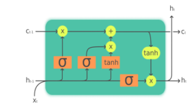Figure 12:  Structure of a LSTM cell

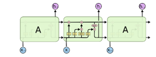Figure 13:  LSTM chain

The calculations that solve the LSTM paradigm are [39]:

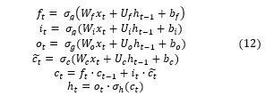where the known data are:

• x_t ϵ R^d– input vector to the LSTM unit,
• d and h – number of input features and number of hidden units, respectively,

Unknowns :

• f_tϵ R^h – forget gate’s activation vector
• i_tϵ R^h – input/update gate’s activation vector
• o_tϵ R^h –  output gate’s activation vector
• h_t ϵ R^h –  hidden state vector (output vector of the LSTM unit)
•  ϵ R^h –  cell input activation vector
• c_t ϵ R_h –  cell state vector
• Wϵ R^hxd ,  U ϵ R^hxd , b ϵ R^h –  weight matrices and bias vector parameters which need to be learned during training

Activation functions are:

• σ_g – sigmoid function
• σ_c – hyperbolic tangent function
• σ_h – hyperbolic tangent function or, linear function

The LSTM training is made in a supervised mode by a set of algorithms like gradient descent, combined with backpropagation through time to compute the gradients needed during the optimization process, in order to change each weight of the LSTM network in proportion to the derivative of the error (at the output layer of the LSTM network) with respect to corresponding weight.  With LSTM units, when error values are backpropagated from the output layer, the error remains in the LSTM unit’s cell. This allows to avoid the problem with standard RNNs where error gradients vanish exponentially with the size of the time lag between important events. The system is trained using the equations (6).

4. Experimental results

The goal of the experiments was to evaluate the four methodologies and find the optimal configuration for each one. The experiments considered only three classes of sounds which could exhaust the specific sounds in the forest environment susceptible to illegal deforestation. They are chainsaw, vehicle, and genuine forest sounds. The identification process was closed set. Segments of 3s were considered and each segment was evaluated individually. We have assessed several lengths of subframes (analysis frames), based on an above remark (see figures 2-4). So, the analysis frames lengths considered are mainly 22ms, 44ms, 88ms. Concerning the frequency interval length, [f_low, f_high], we have investigated lengths of 3.7, 7.4, 10 and 12 kHz. We have conducted these experiments using the MATLAB framework.

The acoustic material contains 99 recordings of the three classes of sounds, in average about 15s each, 39 were used for training and 60 for testing. The testing set resulted in 685 segments of three seconds. The performance of each of the approaches we tested is presented subsequently. The performance was evaluated in terms of Identification rate, the ratio of numbers of correctly identified segments and the evaluated segments.

4.1. MFCC-GMM

We have applied GMM on the feature space consisting of Mel-cepstral features, accompanied or not by ZCR and Spectral Flatness. We have tested several hierarchical clustering initialization methods, using different distance measures between branches, varied the number of Gaussian components, the number of the cepstral coefficients, the values of the frequency interval  [f_low, f_high], and the length of the analysis frame. On the given acoustic material, the performance obtained with the PNN initialization, using the Euclidian Standardized distance, were slightly better than when using the other hierarchical methods. The MATLAB settings for analysis frame, 25ms,  f_low =300 Hz, f_high=3.7 kHz are the most beneficial. Moreover, adding ZCR and SF improved the results. 12-13 GMM components and 13-14 MFCCs seemed to be the best configuration. Some results are presented in Table 1. We have chosen to assign an identical  number of Gaussian components, as our acoustic material is currently quite scarce, and  the investigated problem is less complex than, for instance, the task of an audio scene recognition. A more rigorous approach should consider the structure of the underlying acoustic feature space, as shown in [40], to assign the number of components to each category of sound.

Table 1: Performance of AESR using the MFCC-GMM approach, with additional ZCR and SF features, different values of f_low and f_high expressed in kHz, number of Gaussian components, number of Mel-cepstral coefficients

	flow	fhigh	Components	Coeficients	Identification Rate
					Chainsaw	Forest	Vehicle	General
Euclidian	0.3	3.7	14	13	66.47	77.16	61.07	68.07
	0.3	4	13	13	61.85	76.72	59.92	66.27
	0	3.7	14	13	67.63	79.31	56.87	67.47
Standardised	0.3	3.7	14	13	62.43	80.17	62.21	68.52
	0.3	3.7	15	13	60.69	80.17	62.21	68.07
	0.3	3.7	15	12	67.63	76.29	61.83	68.37

4.2. Spectra Alignment using Dynamic Time Warping

On applying DTW we have aligned Fourier Power Spectra. More precisely, we have aligned segments of these spectra defined on frequency intervals [f_low, f_high]. The frequency domain was restricted to some intervals included in [0, 7400] Hz. The length of the analysis window was set to 22ms. For analysis frames of 22ms the number of samples per frame, given the sampling frequency of 44.1 kHz, is 970, and the length of the Fourier Transform is the closest power of 2 greater than the number of signal samples, that means 1024. For shorter frequency intervals the corresponding Fourier subset involves less samples, less data to be processed, and a shorter execution time:

• [0, 7400] Hz – 171 samples;
• [0, 3700] Hz – 86 samples;
• [300, 3700] Hz – 80 samples;
• [300, 7400] Hz – 165 samples.

For this reason, the length of the analysis frame was set to 22ms. A 25ms frame would have meant a 2048 long Discrete Fourier Transform, and hence, power spectrum.

We have compared the performance of the DTW alignment for several lengths of the frequency interval  [f_low, f_high], different lengths of the Sakoe- Chiba band, and the two distance measures in the calculus of the distortion measure, the Euclidian norm, and the 1-norm (sum of absolute values). The best results for analysis frames of 22ms,  f_low=0,  f_high=7.4 kHz, for the largest applied Sakoe- Chiba band, and the 1-norm. Some of the results can be viewed in the table 2.

Table 2: AESR Performance Using Dynamic Alignment of Power Spectra intervals of various lengths and applying Saloe-Chiba windows endowed with different widths

distance	Sakoe band	flow	fhigh	Identification Rate
				Chainsaw	Forest	Vehicle	General
Norm1	15	0	7.4	69.57	74.14	67.94	70.44
		0	3.7	57.39	81.9	67.94	69.06
	20	0	11	50.43	76.72	67.94	65.19
		0	7.4	68.7	75.86	67.94	70.72
		0	3.7	57.39	83.62	67.94	69.61
	25	0	3.7	57.39	84.48	67.94	69.89
		0	7.4	68.7	76.72	67.94	70.99
	30	0	7.4	69.57	76.72	67.94	71.27
		0	3.7	57.39	86.21	67.94	70.44
Standardised	20	0	3.7	58.26	86.21	66.41	70.17
		0	7.4	68.7	76.72	67.18	70.72
	25	0	3.7	58.26	87.07	66.41	70.44
		0.3	7.4	66.09	77.59	67.18	70.17
		0	7.4	68.7	77.59	67.18	70.99
	30	0	7.4	68.7	77.59	67.18	70.99

4.3. Experiments using the FFNN

We have applied FFNN methodology in two hypostases: the first by feeding at input Mel-cepstral features (coming with or without Spectral Flatness, and/or ZCR) and the second, by feeding Fourier power spectrum features. In the first case we have extracted 12 to 20 Mel-cepstral coefficients, on an analysis window, using different frequency intervals [f_low, f_high], and different analysis window lengths. In the second case the number of coefficients depended on the length of the frequency interval.

At training we fed the information at the of sample level, each sample being associated with the expected outputs 1, 0 or -1, depending on the nature of the sound sample (chainsaw, genuine forest, vehicle engines). A sample in this case means a feature vector (of Mel-cepstral coefficients or Fourier spectrum coefficients, etc., calculated on an analysis window).

We applied the batch training and evaluated the BR, and LMA training algorithms. At classification, when training by feeding vectors of features, we evaluated each 3s segment by assessing each sample in the segment and finally the whole segment.  A sample belongs to a certain class if its output score in (11) is closest to the respective class expected output, 1, 0 or -1. The overall decision on the 3s level is taken by applying one of the rules:

• Majority voting (the segment is associated with the class for which most of the samples of the segment belong to the respective class);
• Average output: the average output score of the samples on the segment is closest to the expected output of a certain class.

Concerning the network architecture, we have tested several configurations of FFNNs, 2 to 4 layers, with 6 to 10 neurons on each layer. As the performance of the test depends on the initialization of the training process, we provided 5 tests for each configuration. Because of the great choice of parameters, such as the length of the analysis window, or f_low, f_high, and configurations to be investigated, we could not exhaust all the possible combinations. The tables 3 and 4 present some relevant results.

Table 3: FFNN – MFCC -results of 5 tests using networks of 4 layers, with 9, 8, 7, 6 neurons respectively 88ms analysis windows, , [f_low, f_high] =[0, 7.4] kHz, 18 Mel-coefficients, and Spectral flatness. Training was accomplished by Bayesian Regularization, and classification using the majority voting rule

	Chainsaw	Forest	Vehicle	General
test1	52.36	93.10	62.69	70.13
test2	51.83	75.86	62.69	64.13
test3	48.69	89.66	60.00	66.91
test4	50.26	81.90	68.46	67.94
test5	58.64	93.10	61.92	71.60

Table 3 shows one the best performance, identification rates expressed in percent, obtained using Mel-cepstral features as input, using a 4 layers FFNN, with 9, 8, 7, 6 neurons on each layer, 88ms analysis windows, [0, 7.4] kHz, frequency interval for which the coefficients were computed. 18 Mel-coefficients were extracted, and Spectral flatness and ZCR added on each analysis frame. Training was accomplished by Bayesian Regularization, the default in MATLAB, and classification using the majority voting rule. The average performance was 68.14%. Similar results were obtained using other configurations, for instance an identification rate of 67.43% was achieved with a 3-layer network, 88ms analysis frame, [f_low, f_high] =[0, 10] kHz,  17 Mel cepstral coefficients, with SF added. However, all the tests provided a low identification rate for the “chainsaw” class. This performance is lower, or comparable to the ones obtained applying the classical GMM and DTW approaches.

Table 4 presents the results of 5 tests using FFNN of 4 layers, with 9, 8, 7, 6 neurons respectively, with Power Spectrum coefficients as input, 88ms analysis windows, [0, 7400] Hz frequency interval for spectral features. At training we applied the Bayesian Regularization algorithm and at classification the majority voting rule. The average performance was 78.82%.

Table 4: FFNN – Power Spectrum – results of 5 tests using networks of 4 layers, with 9, 8, 7, 6 neurons respectively, 88ms analysis windows, [f_low, f_high] =[0, 7.4] kHz, training models obtained by Bayesian Regularization and classification using the majority voting rule

	Chainsaw	Forest	Vehicle	General
test1	74.86	92.24	74.61	80.67
test2	65.96	91.37	78.46	79.35
test3	78.01	87.06	77.69	80.96
test4	67.53	80.17	78.46	75.98
test5	75.39	77.58	78.07	77.16

Tables 5 and 6 present some relevant results obtained using the LMA algorithm at training.

Table 5 presents the identification rate (in percent) of 5 tests using a 4-layernetwork, an analysis frame of 88ms, [f_low, f_high] =[0, 10] kHz,  18 Mel cepstral coefficients, without adding extra parameters. At classification, the majority voting rule was applied. The average achieved performance was 69.54%.

Table 5: FFNN – MFCC -results of 5 tests using networks of 4 layers, with 9, 8, 7, 6 neurons respectively 88ms analysis windows, , [f_low, f_high] =[0, 10] kHz, 18 Mel-coefficients. Training was accomplished using LMA, and classification using the majority voting rule

	Chainsaw	Forest	Vehicle	General
test1	58.12	90.52	70.77	73.94
test2	52.36	85.35	65.39	68.52
test3	44.50	87.07	75.00	70.57
test4	40.31	76.72	67.31	62.96
test5	49.74	87.93	72.31	71.30

Table 6 presents the results of 5 tests using networks of 3 layers, with 9, 8, 7 neurons respectively, 88ms analysis windows, and the frequency interval [0, 3700] Hz, applying LMA training and classification using the majority voting rule. The average recognition rate was 79.17%.

Table 6: FFNN applied on Power Spectra results of 5 tests using networks of 3 layers, with 9, 8, 7 neurons respectively, 88ms analysis windows, , [f_low, f_high] = [0, 3700] Hz, training models obtained by LMA and classification using the majority voting rule

	Chainsaw	Forest	Vehicle	General
test1	72.77	84.48	77.69	78.62
test2	75.39	79.31	85.76	80.67
test3	69.11	89.65	69.23	76.13
test4	69/63	90.08	79.61	80.38
test5	64.92	87.93	84.23	80.08

Table 7: FFNN applied on Power Spectrum results of 5 tests using networks of 4 layers, with 10, 9, 8, 7  neurons respectively, 88ms analysis windows, [f_low, f_high] = [0, 3700] Hz, training using LMA and classification and the average score on the 3s frames

	Chainsaw	Forest	Vehicle	General
test1	50.26	92.24	65.769	70.42
test2	61.25	95.69	70.769	76.57
test3	43.97	94.82	65.00	69.25
test4	53.40	93.10	70/38	73.35
test5	57.59	98.27	62.30	73.20

Table 8: Average Identification rates obtained using FFNN applied on Power Spectra, with 3 layers with 9, 8, 7 neurons, respectively,  using different values for f_high  and lengths of the analysis frame, training with Bayesian  Regularization and majority vote classification.

		analysis frame lengths
		22ms	44ms	88ms
Frequency interval (Hz)	[0, 3700]	71.04	76.31	78.83
	[0, 7400]	74.98	76.02	77.22
	[0, 10000]	69.64	74.76	76.02
	[0, 12000]	72.61	75.17	74.00

Table 7 contains the results of 5 tests applying FFNN to spectral coefficients, calculated on the frequency domain [0, 3.7] kHz, using a 88ms analysis windows, and applying the LMA training on 4-layer networks with 10, 9, 8, 7 neurons. The classification algorithm used the average score on 3s frames. The average performance was 72.56%.

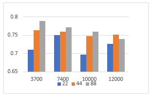Figure 14:  Average Identification rates for different values of f_high and length of the analysis frame

As an overall conclusion of the results, the Fourier spectrum as input to FFNN yielded very good results when applying the classification majority vote rule. The average score rule produced poorer results, with a low performance for the “chainsaw” class,  but they are still better than using Mel-cepstral analysis or the GMM and DTW approaches. The BR and LMA produced comparable results, maybe LMA results were more balanced among the 5 tests (the standard deviation among the identification rates is lower). Concerning the network architecture for the Fourier spectrum variants of 2, 3 or 4 layers produce comparable results, especially when using the majority voting rule. The LMA training resulted in performance quite similar results as those obtained using the BR, for many configurations besides the one illustrated in Table 6, and the results are well balanced among the three classes of sounds. Perhaps the identification rates for the “chainsaw” class are a bit lower. In what concerns the average score classification, the 3 layers FFNN seemed to work better than 4-layer nets.

Concerning the analysis window, the results are better in all the cases for lengths of 44ms or 88ms. Table 8 and Figure 14 present the average overall identification rates for the FFNN applied on power spectra using the BR training, and majority voting at classification, several analysis window lengths and frequency intervals. The best average score is obtained for  the spectrum restricted to [0, 3700]Hz, and an analysis window of 88ms, but in fact the results are very close among the frequency intervals. Among the 5 tests for each configuration there were many  identification rates above 80%.

With regard to the results obtained using the Mel-cepstral coefficients as input, the conclusion concerning the optimum analysis window length is that window lengths greater than 44ms produced better performance. The frequency intervals [0, 7.4] kHz and [0, 10] kHz yielded better results. The general conclusion is that adding Spectral flatness and sometimes ZCR helped to increase the performance, although the example of Table 5 is an exception.

4.4. Experiments using the LSTM

In the experiments using LSTM we used the same input as in the FFNN experiments. The number of hidden units was set to 100 and each cell configured with 5 layers, the default MATLAB configuration. Table 9 presents the best results obtained so far by applying LSTM. We have fed as input 18 dimensional sheer Mel-cepstral vectors, calculated on 44ms analysis window and filtering the frequency domain to [0, 12] kHz. The average performance among the 5 tests is 64.85%.  As can be seen the identification rates are unbalanced among the three classes. In any other configurations the results were even worse.

Table 9: Results of 5 tests using LSTM applied on an input set of Mel-cepstral 18-dimensional vectors, calculated on 44ms analysis windows, and the frequency interval of [0, 12] kHz

	Chainsaw	Forest	Vehicle	General
test1	48.69	86.20	47.69	61.05
test2	37.69	93.10	56.92	63.83
test3	42.40	97.41	45	62.07
test4	67.53	90.51	47.69	67.78
test5	62.82	93.10	53.46	69.54

Concerning the experiments using as input the Fourier spectrum we failed to obtain interesting results, as the network did not behave well at training Figures 15, 16 present the estimation of the achieved accuracy during the training process for LSTM applied to Mel-cepstral input and power spectra respectively. While the first process achieves maximum accuracy in less than 100 iterations the LSTM applied to power spectra achieves less than 80% in more than 300 iterations.

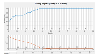Figure 15:  Accuracy estimation during training for a LSTM – MFCC process

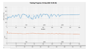Figure 16: Accuracy estimation during training for a LSTM applied on Fourier power spectra.

Regarding the experiments using as input the Fourier spectrum we failed to obtain interesting results, as the network did not behave well at training Figures 15, 16 present the estimation of the achieved accuracy during the training process for LSTM applied to Mel-cepstral input and power spectra respectively. While the first process achieves maximum accuracy in less than 100 iterations the LSTM applied to power spectra achieves less than 80% in more than 300 iterations.

5. Conclusions and future work

The goal of this study was to test some state-of-the-art methodologies applied in AESR, Gaussian Mixtures Modelling, Dynamic Time Warping, and two types of Deep Neural Networks, in the context of forest acoustics.  Another specific objective was to evaluate the behaviour of these techniques, in several configurations, such as different lengths of the analysis window, or find the frequency intervals on which the Fourier spectrum is more relevant for such type of applications.

We have succeeded to achieve significantly better performances using Feed Forward Neural Networks, in a certain setup, compared to the classical methods, GMM, and DTW. We used two types of networks (Deep Feedforward Neural Network and LSTM) and have fed as inputs two types of data, Mel-cepstral and Fourier power spectral coefficients. In this context we tested two training methods, the Levenberg-Marquardt Algorithm, and the Bayesian Regularization, and two different classification approaches.

Deep Feed Forward Neural Networks experiments output the best results when using the sheer spectral features, and especially when using the majority voting rule, with an average identification rate of over 78%, with about 10% higher than other methods performance. This fact suggests that FFNN, based on Fourier spectral features, using a less complex processing sequence, is able to produce more valuable features than the elaborate Mel cepstral analysis. A difference is in the number of features at input, while the Mel features are fewer than 20, the spectrum on [0, 7400] Hz frequency interval means about 170 coefficients.

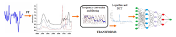Figure 17:  FFNN using Mel cepstral input applies a range of transforms (frequency conversion. spectrum filtering, logarithm, Discrete Cosinus Transform) on the Fourier spectrum and feeds the result to the network

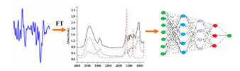Figure 18:  FFNN using Fourier Spectrum coefficients as has a simpler schema, and probably devises more valuable features through the layers of the network

Figures 17, 18 summarize this idea. Figure 17 presents the more complex row of operations to be accomplished on the power spectrum when the input to the FFNN involves Mel-cepstral analysis. Figure 18 presents the straightforward processing of spectrum by the FFNN, when just spectral coefficients are fed to the network.

The disappointing results using the LSTM network may have several reasons. One of them may be the unproper use of the LSTM MATLAB tool. A second reason may reside in the fact that this type of network might be not suited to the kind of problem we want to solve.

Another advantage of using FFNN is the fact that it is easy to implement in programming environments other than MATLAB. While the models can be generated in MATLAB, the classification part can be implemented in other programming languages, like C++, Java, etc. using the parameters established at training.

Concerning the length of the analysis window the experimental results have shown that its length must be set above 44ms or higher. We have chosen the length of the analysis window somehow empirically, therefore the use of an analytical approach, e.g., [41], to establish the proper length of the frame would be a future direction of research.

We could not draw a well-founded conclusion about the optimal frequency interval, as for 3.7 kHz to 10 kHz, the results do not vary too much.

Although the neural networks have apparently the advantage of  training jointly several classes of data, this did not result in better results in comparison with the classical methods.

As future work we intend to extend our research by including the CNN framework.

Another important objective would be investigation of methods to merge decision of several sources, possibly by using a probabilistic logic.

Another important objective is to extend the field of research to other AESR applications, in the field of scientific environment monitoring (e.g., detect bird or species), or early detection of disasters such as land sliding or avalanches, where acoustic emissions are among the data used as input.

Conflict of Interest

The authors declare no conflict of interest.

Acknowledgment

This work has been supported in part by UEFISCDI Romania through projects SeaForest, CitiSim, SenSyStar and WINS@HI, and funded in part by European Union’s Horizon 2020 research and innovation program under grant agreement No. 777996 (SealedGRID project) and No. 643963 (SWITCH project).

1. S. Segarceanu, E. Olteanu, G. Suciu, “Forest Monitoring Using Forest Sound Identification,” in 2020 International Conference on Telecommunications and Signal Processing (TSP-2020), 346-349 2020, doi: 10.1109/TSP49548.2020.9163433.
2. S. Cowling, M. Cowling, R. Sitte, “Recognition of Environmental Sounds Using Speech Recognition Techniques,” Advanced Signal Processing for Communication Systems, 31-46, 2006, doi : 10.1007/0-306-47791-2_3.
3. X. Guo, Y. Toyoda, H. Li, J. Huang, S. Ding, Y. Liu, “Environmental Sound Recognition Using Time-Frequency Intersection Patterns,” Applied Computational Intelligence and Soft Computing, vol. 2012, 6 pages, 2012, https://doi.org/10.1155/2012/650818.
4. S. Sivasankaran, K.M.M. Prabhu, “Robust features for Environmental Sound,” in 2013 IEEE Conference on Electronics, Computing and Communication Technologies (CONECCT), 1-6, 2013, doi:10.1109/CONECCT.2013.6469297.
5. S. Sigtia, A. Stark, S. Krstulovic, M. Plumbley, “Automatic environmental sound recognition: Performance versus computational cost,” IEEE/ACM Transactions on Audio, Speech, and Language Processing, 24(11). 2096-2107, 2016, doi: 10.1109/TASLP.2016.2592698.
6. M. Babiš, M. Ďuríček, V. Harvanová, M. Vojtko, “Forest Guardian –Monitoring System for Detecting Logging Activities Based on Sound Recognition,” in 2011 7th Student Research Conference in Informatics and Information Technologies, 2, 354-359, 2011.
7. J. Papán, M. Jurecka, J. Púchyová, “WSN for Forest Monitoring to Prevent Illegal Logging,” in 2012 IEEE Proceedings of the Federated Conference on Computer Science and Information Systems, 809-812, 2012.
8. R. Buhuș, L. Grama, C. Rusu, 2017, “Several Classifiers for Intruder Detection Applications,” in 2017 9th International Conference on Speech Technology and Human-Computer Dialogue (SpeD), 2017, doi: 10.1109/SPED.2017.7990432.
9. L. Grama, C.Rusu, “Audio Signal Classification Using Linear Predictive Coding And Random Forest,” in 2017 9th International Conference on Speech Technology and Human-Computer Dialogue (SpeD), 1-9, 2017, doi: 10.1109/SPED.2017.7990431.
10. S. Zhang, D. Gao, H. Lin, Q. Sun, “Wildfire Detection Using Sound Spectrum Analysis Based on the Internet of Things,” in 2019 Sensors, 19(23), 2019, doi: 10.3390/s19235093.
11. L. A.Venier, M. J. Mazerolle, A. Rodgers, K. A. McIlwrick, S. Holmes, D. Thompson, “Comparison of semiautomated bird song recognition with manual detection of recorded bird song samples,” Avian Conservation and Ecology, 12(2), 2017, doi:10.5751/ ACE-01029-120202.
12. D. Mitrovic, M. Zeppelzauer, C. Breiteneder, “Discrimination and Retrieval of Animal Sounds,” in 2006 12th International Multi-Media Modelling Conference. IEEE, 2006, doi: 10.1109/MMMC.2006.1651344.
13. S.Chandrakala, S. Jayalakshmi, “Environmental Audio Scene and Sound Event Recognition for Autonomous Surveillance: A Survey and Comparative Studies,” ACM Computing Surveys, 52(3), 1-34, 2019, doi: 10.1145/3322240.
14. N. Dixon, A., Smith, J. A. Flint, R. Khanna, B. Clark, M. Andjelkovic, “An acoustic emission landslide early warning system for communities in low-income and middle-income countries,” Landslides, 15, 1631–1644, 2018, doi:10.1007/s10346-018-0977-1.
15. Z. M. Hafizi, C.K.E. Nizwan, M.F.A. Reza & M.A.A. Johari, “High Frequency Acoustic Signal Analysis for Internal Surface Pipe Roughness Classification,” Applied Mechanics and Materials, 83, 249-254, 2011, doi:10.4028/www.scientific.net/AMM.83.249.
16. V. Gibiat, E. Plaza, P. De Guibert, “Acoustic emission before avalanches in granular media,” The Journal of the Acoustical Society of America, 123(5), 3270, 2008,doi: 10.1121/1.2933600 .
17. T. Thüring, M. Schoch, A. van Herwijnen, J. Schweizer, “Robust snow avalanche detection using supervised machine learning with infrasonic sensor arrays,” Cold Reg. Sci. Technol., 111, 60–66, 2015. doi: 10.1016/j.coldregions.2014.12.014
18. L. G. Evers, D. Brown, K. D. Heaney, J. D. Assink, P. S.M. Smets, M.Snellen, “Infrasound from underwater sources,” The Journal of the Acoustical Society of America, 137(4), 2372-2372, 2015, doi: 10.1121/1.4920617.
19. M. Cowling, R Sitte, T. Wysock, “Analysis of Speech Recognition Techniques for use in a Non-Speech Sound Recognition System,” Advanced Signal Processing for Communication Systems. Springer, 2002.
20. S. Chachada, C.-C. Jay Kuo , “Environmental Sound Recognition: A Survey,” APSIPA Transactions on Signal and Information Processing, 3, 2014, doi: 10.1109/APSIPA.2013.6694338.
21. I. V. McLoughlin, Hao-min Zhang, Zhi-Peng Xie, Yan Song, Wei Xiao, “Robust Sound Event Classification using Deep Neural Networks. Audio, Speech, and Language Processing,” IEEE/ACM Transactions on Audio, Speech and Language Processing, 23 (3). 540-552, 2015, doi:10.1109/TASLP.2015.2389618) (KAR id:51341.
22. T. Lidy, A. Schindler, “CQT-based convolutional neural networks for audio scene classification,” in 2016 Proceedings of the Detection and Classification of Acoustic Scenes and Events Workshop (DCASE’16), 90, 1032-1048. doi: 10.1145/3322240.
23. A. Rabaoui, M. Davy, S. Rossignol, N. Ellouze, “Using one-class SVMs and wavelets for audio surveillance,” IEEE Trans. on Information Forensic and Security, 3(4), 763–775, 2008, doi: 10.1109/TIFS.2008.2008216.
24. D. Stowell, D. Clayton., “Acoustic event detection for multiple overlapping similar sources,” in 2015 Proceedings of the IEEE Workshop on Applications of Signal Processing to Audio and Acoustics (WASPAA’15). 1–5, 2015, doi: 10.1109/WASPAA.2015.7336885.
25. H. Phan, P. Koch, L. Hertel, M. Maass, R. Mazur, A. Mertins, “CNN-LTE: A class of 1-X pooling convolutional neural networks on label tree embeddings for audio scene classification,” in 2017 Proceedings of the International Conference on Acoustics, Speech, and Signal Processing (ICASSP’17), 136-140, 2017, doi: 10.1109/ICASSP.2017.7952133.
26. Karol J. Piczak, “Environmental sound classification with convolutional neural networks,” in 2015 IEEE 25th International Workshop on Machine Learning for Signal Processing (MLSP), 1–6, 2015, doi: 10.1109/MLSP.2015.7324337.
27. Y. Han, K. Lee, “Convolutional neural network with multiple-width frequency-delta data augmentation for acoustic scene classification,” in 2016 Proceedings of the IEEE AASP Challenge on Detection and Classification of Acoustic Scenes and Events, 2017.
28. R. Ahmed, T. I. Robin, A. A. Shafin, “Automatic Environmental Sound Recognition (AESR) Using Convolutional Neural Network,” International Journal of Modern Education and Computer Science, 12(5), 41-54, 2020, doi: 10.5815/ijmecs.2020.05.04.
29. H. Eghbal-zadeh, B. Lehner, M. Dorfer, G. Widmer, “A hybrid approach with multichannel i-vectors and convolutional neural networks for acoustic scene classification,” in 2017 25th European Signal Processing Conference (EUSIPCO), 2749-2753, 2017, doi: 10.23919/EUSIPCO.2017.8081711.
30. D. Reynolds, “Gaussian mixture models,” Encyclopedia of Biometrics, 659–663, 2009, doi:10.1007/978-0-387-73003-5_196.
31. X. Huang, A. Acero, H. Hon, Spoken Language Processing:A Guide to Theory, Algorithm, and System Development, Prentice Hall, 2001.
32. O.Virmajoki, P. Fränti, “Fast pairwise nearest neighbor based algorithm for multilevel thresholding,” Journal of Electronic Imaging, 12(4), 648-659, 2003, doi: 10.1117/1.1604396.
33. S. B. Davis, P. Mermelstein, “Comparison of parametric representations for monosyllabic word recognition in continuously spoken sentences,” IEEE Trans. on ASSP, 28, 357–366, 1980, doi: 10.1109/TASSP.1980.1163420.
34. S. Furui, “Cepstral analysis technique for automatic speaker verification,” IEEE Transactions on Acoustics, Speech, and Signal Processing, 29, 254–272, 1981, doi: 10.1109/TASSP.1981.1163530.
35. P. Senin, “Dynamic Time Warping Algorithm Review,” Technical Report Information and Computer Science Departament University of Hawaii, 2008.
36. H. Sakoe, S. Chiba, “Dynamic programming algorithm optimization for spoken word recognition,” Trans. Acoustics, Speech, and Signal Proc., 26, 43-49, 1978, doi:10.1109/TASSP.1978.1163055.
37. V. Zacharias, AI for Data Science Artificial Intelligence Frameworks and Functionality for Deep Learning, Optimization, and Beyond, Technics Publications, 2018.
38. M. H. Beale, M. T.Hagan, H. B. Demuth, Neural Network Toolbox™ User’s Guide, The MathWorks, Inc., Natick, Mass., 2010.
39. H. Sak, A. Senior, F. Beaufays, “Long short-term memory recurrent neural network architectures for large scale acoustic modeling,” in 2014, Fifteenth annual conference of the international speech communication association (INTERSPEECH-2014), 338-342, 2014.
40. M. Kuropatwiński, “Estimation of Quantities Related to the Multinomial Distribution with Unknown Number of Categories,” in 2019 Signal Processing Symposium (SPSympo), 277–281, 2019, doi:10.1109/sps.2019.8881992.
41. E. Punskaya, C. Andrieu, A. Doucet, W. Fitzgerald, “Bayesian curve fitting using MCMC with applications to signal segmentation,” IEEE Transactions on signal processing, 50(3), 747-758, 2002, doi: 10.1109/78.984776.

(Click Here)