1. Introduction

This paper (hereinafter the “extended paper”) is an extension of the report presented at the 2020 IEEE 2nd International Conference on System Analysis_Intelligent Computing (SAIC) held in Kyiv, Ukraine, in October 2020 [1] (hereinafter the “conference paper”). The conference paper was a byproduct, on a sideline, of the other series of our research [2–7], which was aimed at finding the origin of the global climate change.

At the beginning of the research [2-5], we assumed that Moon’s gravity could be related to the increase of the global temperature, then we calculated the coefficients of several variables such as the distance between Moon and Earth, the global temperature, the emitted carbon dioxide, with the method of econometrics, regarding the distance between Moon and Earth as the surrogate for the energy of the Moon’s gravitational field and gravitational waves. Then we reached an assumption that there should be anti-gravitational waves as the antimatter of graviton (gravitational waves) similar to positron as the antimatter of electron; and, we derived the equation of motion of anti-gravitational waves, upon the equation of motion for gravitational waves [8] that was predicted in the flat surface in the rectilinear coordinate system, approximating the special theory of relativity. Then we reported the result of our analysis in a paper [6]. The geometrical relation between the positive and negative flows of gravitational waves (gravitational and anti-gravitational waves) that we made for [6] is shown in Figure 1.

The next question was “How can both positive and negative flows be created?” Then we reviewed the general theory of relativity [8] that explained the gravitational field by the following equations:

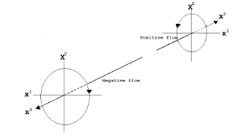Figure 1: Geometrical relation between positive and negative flows of gravitational waves [6]

    is called the Ricci tensor, which is a variation of the curvature tensor, and  is called a Christoffel symbol. Also, is called the fundamental tensor that makes the Christofell symbol. The equation (3) shows how the fundamental tensor describes a four-dimensional space-time. Here, the notation for the differential of the tensor is given by , where F is any function such as  and/or , and  is the  variable (vector) in the given coordinate system.

The fundamental tensor also makes a geodesic, a path of extremal distance, as shown below.

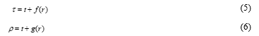
In the equation (4),  is time,    is the mass of a planet, is the distance from the planet,    is the angle from the axis of , and  is the angle of the rotation around the axis of  in the spherical polar coordinate system. In (3), there is a singularity at : therefore, the space is divided into two regions, and . In the region of , the mass of the planet must be very dense and heavier and it can be a black hole. To connect these two regions, a different coordinate system was invented [8], which makes the distorted time, , and the distorted distance, , by the following equations:

The section 2.2. describes how this idea is taken into account in the numeric simulation.

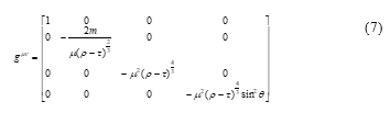
Then the equation (3) was transformed to the equation (7).

Then the geodesic was also transformed from (4) to (8).

The followings show how to make (1) and (2) by the fundamental tensor:

For example, if ,

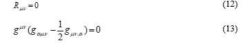
According to [8], in the empty space where only the gravitational field of a planet exists, becomes zero as shown in (12); then (13) is the equation of motion of a particle.

Then in order to describe gravitational waves moving in the gravitational field, the equation of motion is differentiated once again as shown below.

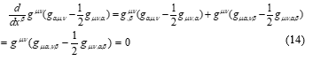
This equation leads to the equation (15), and this is the equation of motion for gravitational waves, according to [8].

The notation for the secondary differential of , for example by the vectors,  and , is .

      Here, we show this equation only for describing how the gravitational field is related to the creation of gravitational waves; although, this extended paper doesn’t include the simulation of gravitational waves.

Then we made the numeric simulation [7] on the curved space, deriving the mathematical forms of the components of the Ricci tensor (1). The following equation is an example of the Ricci tensor in case of , , :

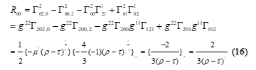      Then we calculated the coefficient of each component of the tensor, for , , , , , , , , , , , , and , , , , using a personal computer. The algorithm to calculate the coefficients is described in the section 2.3.

After making the numeric simulation [7] with the curvature tensor, there was still a need to confirm the negative flow of gravitational waves that are to be created by some movement of a strong gravity; however, we could not find any suitable physical object that could be referred to. Therefore, we invented an idea of  the hypothetical rotation of an artificial object shown in Figure 2 as a possibility of the movement of a strong gravity. Then we reported the result of the simulation in the conference paper [1] as the “theory and simulation of artificial antigravity”.

While the conference paper [1] has reported the result of the simulation on the gravitational energy made by rotating the very strong gravity, this extended paper reports one more feature, the angular momentum, by which we attempt to examine whether there is a consistent explanation of anti-gravitational waves shown in Figure 1, or not.

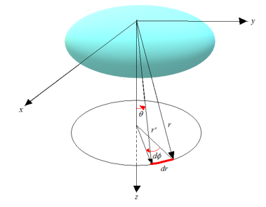Figure 2: Rotation of an object

It is noted that there is no data taken out from any experiments in laboratories or observations in the cosmos, but this research is made solely on the mathematical model taken out from the general theory of relativity [8] as well as the classical mechanics [9].

For the numeric simulation, we used a personal computer’s software, which was developed for the econometrics of geometry [10]. The algorithm of this software was originally developed in the rectilinear coordinate system; but, we used it for calculating the coefficients of the equation of motion in the spherical polar coordinate system as a special case of the curved space. In other words, we used the function of the orthogonal transformation of the matrix algebra as the surrogate for the tensor algebra needed in the general theory of relativity.

2. Method

2.1. Curvature Tensor before the Rotation

For the simulation of this extended paper, we used the same curvature tensor shown in (17) that we used for our previous research for the conference paper [1]. This tensor is for simulating the gravitational field before the rotation. From it, we took the components of ,  and  for simulating the spatial movement of the object, but excluded  from the simulation because it is for the distorted time coordinate, which is beyond the scope of this research.

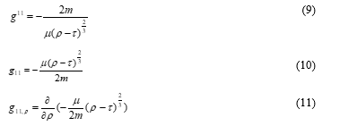
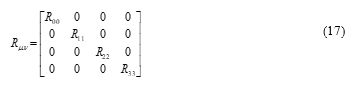The diagonal components of are shown in the equations from (18) to (21), which are taken from our previous research [7].

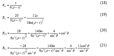 is given by the following equation with the mass of a planet, :

2.2. Distortion of time and space in strong gravity

We used the same assumption of our previous research [1] for simulating the distortion of time and space, as shown in Figure 3 and Figure 4. In these figures,  is the distance from the center of the strong gravity,  is the time to travel for the distance,  is the  distorted time (5), which expands and shrinks depending on the distance  and the time ; and, is the distorted distance (6), which expands and shrinks depending on the time  and the distance .

For the simulation, we created two models, Case-1 (non-linear model) and Case-2 (linear model) as shown in Table 1, which assign the functions of in the equation (5) and  in the equation (6).

Table 1: Two models for simulating the distorted time-space

	Case-1 (Non-linear model)	Case-2 (Linear model)

Then we made the distributions of  and , following the description of [8], “Any signal, even a light signal, would take an infinite time to cross the boundary of a black hole”. However, we could not set the infinite values for the simulation; therefore, instead we set 24 discrete finite values in order to mock “It takes more time to travel closer to the center of the black hole”. The values of  and  are assigned to make input vectors for the numeric simulation with a personal computer.

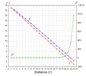Figure 3: Time and distance from the center of the gravity, Case-1 (non-linear distortion): and

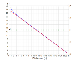Figure 4: Time and distance from the center of the gravity, Case-2 (linear distortion): and

2.3. Algorithm for the gravitational energy with no rotation

We used the same algorithm that we used for our previous research [1] to calculate the relative intensity of the gravitational energy with the curvature tensor, which was to be reflected by the stress-energy tensor placed at the end of the distance ϒ in Figure 3 and 4.

The Einstein’s equation that rules the motion of particles in the gravitational field is shown below.

Then we took the idea of the stress energy tensor from the classical mechanics [9] and set the equation (24), where T is the stress energy tensor and  is a constant.

      In order to calculate the coefficients of the tensor, we made the equation shown below, where ,  and  are the coefficients that make a column vector, .

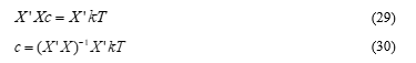
For calculating , we formed a  matrix, , by three vectors, ,  and , as shown in (26) for making the projected image of the gravitational energy on the surface of the sphere in the spherical polar coordinate system.

To solve this equation, we set the constraint (28), where  is the transposed matrix of .

 (28) The matrix algebra continues as shown in (29) and (30) to calculate the values of .

      The standard errors of the coefficients are also calculated by (31) , where  is the variance of the .

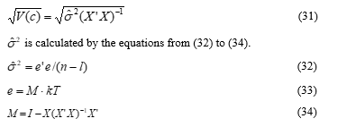 is the number of rows of each column of , while in this simulation the value of  is 23 as shown in Figure 3 and 4.  is the number of columns of , and  is a  unit matrix that holds 1 (unity) in all diagonal components and 0 in the other components.  is the inverse matrix of , and  is the transposed vector of .

2.4. Algorithm for the gravitational energy with rotation

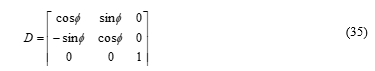
If the object rotates as shown in Figure 2, its coordinate system is transformed by the transformation matrix  of the Euler’s angles [9] shown below.

For the rotation of the object around one axis of , the tensor of the object’s coordinate system, , is multiplied by ; then it is transformed as shown below.

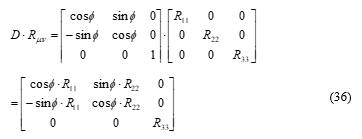The components,  and  are anti-symmetrical, which are perpendicular to the rotation axis,  for  of Figure 2. From the above transformed tensor after the rotation, , we took out its diagonal components and formed (37), to calculate the relative intensity of the principal moment of the rotation.

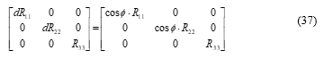
Then we formed  as shown below to calculate the coefficients of the diagonal components.

Henceforth we followed the same procedure explained in the section 2.3., but with the matrix shown below.

2.5. Algorithm for the angular momentum of the rotation

      We formed a matrix shown in (40), by taking out the anti-symmetrical components of from (36); then formed a column vector shown in (41).

With the above column vector, we formed  shown below, for calculating the coefficients of the vector’s components.

Then we followed the same procedure as explained above, but with the matrix shown in (43) of the anti-symmetrical components. It is to simulate the angular momentum that is to be projected on the imaginary flat surface, which is perpendicular to the spherical surface.

here a little explanation is needed about  of (43). At first,  of (44) is an infinitesimal rotation operator. But, in general it has a form of (45) according to the Reference [9]. Then a rotated vector as the cross-product of and  makes (46).

However, in this simulation, we assumed (47) and (48), which make (41) instead of (46).

2.6. Input data

The time  and the distance  are set as shown in Figure 3 for Case-1 and in Figure 4 for Case-2. For simulating the spatial expansion of the gravitational field, we assumed as if  would become larger in far distance as shown in Figure 5. For simulating the rotation of the object, we set two cases, assuming  (the rotation 1) and  (the rotation 2) also as shown in Figure 5. With these settings, , , , , ,  and  behave as shown in Figure 6.

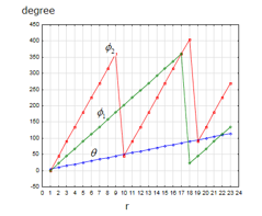Figure 5: Angles, ,  and , for the simulation

In addition, we set the stress-energy tensor as 1; because, the purpose of this simulation is to measure the relative intensity of each component of the tensors.

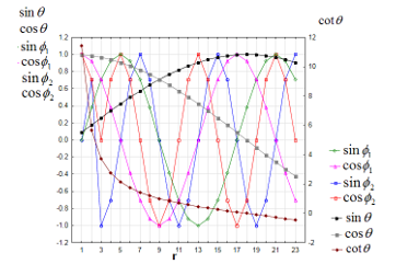Figure 6: , , ,   , ,  and

3. Result

3.1. Gravitational energy and angular momentum: overview

Figure 7 (Table 2) shows the relative intensity of the gravitational energy of the object, which is projected on the surface of the sphere of the curved space, and the angular momentum of the perpendicular vector to the surface. In Case-1 (non-linear distortion of the time and space), the gravitational energy (on curved surface) is negative (gravity) before the rotation, but it changes to positive (antigravity) in the rotation 1, and then to negative (gravity) again in the rotation 2. It means that the antigravity appears, depending on the speed of the rotation of the object. The sign of the angular momentum (on perpendicular vector) changes from positive to negative when the rotation becomes faster (from the rotation 1 to the rotation 2). It means that the direction of the angular momentum changes, depending on the speed of the rotation. In Case-2 (linear distortion of time and space), the gravitational energy is positive with no rotation (but smaller than in Case-1 and closer to zero) in Figure 7; while, the gravitational energy (negative) becomes larger when the object rotates faster. The angular momentum of Case-2 changes as it changes in Case-1.

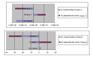Figure 7: Gravitational energy on curved surface and angular momentum on perpendicular direction to the surface

Note: In Figure 7, “On curved surface” means the gravitational energy, which is the sum of the calculated coefficients in the equation of (25) for the no rotation and the sum of the calculated coefficients in the equation of (38) for each of the rotation 1 and the rotation 2. “On perpendicular vector” means the angular momentum, which is the sum of the calculated coefficients of (42) for each of the rotation 1 and the rotation 2.

Table 2: Intensities of gravitational energy and angular momentum: overview

	Case-1		Case-2
	On curved surface	On perpendicular vector	On curved surface	On perpendicular vector
No rotation	-78.55	—	1.770	—
Rotation 1	20.00	36.90	-8.178	14.77
Rotation 2	-41.96	-43.00	-21.31	-15.29

3.2. Gravitational energy in three directions

Figure 8 (Table 3) and Figure 9 (Table 4) show the intensities of the gravitational energy, projected on the spherical curved surface in the components of ,  and  with no rotation, and in the components of ,   and  with the rotation 1 and the rotation 2.

In Figure 8 for Case-1, only the component of  appears on the surface with no rotation, and only the component of appears with the rotation 1 and the rotation 2. The rotation 1 shows the antigravity (positive).

In Figure 9 for Case-2, the component of  also appears in addition to the component of when the object rotates, and they become positive (antigravity) with the rotation 1 and the rotation 2. Here, it is noted that the components of  and   don’t appear in Case-1 of Figure 8, but their calculated values are shown in Table 3; and, in Case-2 the component of  doesn’t appear in Figure 9, but its calculated values are shown in Table 4.

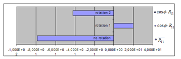Figure 8: Projection of the gravitational energy in 3 directions on the surface of the curvature, Case-1

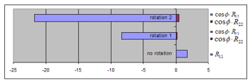Figure 9: Projection of the gravitational energy in 3 directions on the surface of the curvature, Case-2

Table 3: Intensity of gravitational energy in 3 components, Case-1

Diagonal components of	c and of before the rotation	Diagonal components of rotated	c and  (Rotation 1)	c and  (Rotation 2)
	-78.68 (26.49)		20.01 (58.22)	-42.05 (52.30)
	0.1307 (0.03369)		-5.516 (0.0803)	0.08903 (0.06829)
	-6.803 (2.557 )		-3.290 (3.869 )	-2.990 (5.403 )

Note: The value without the bracket is the coefficient c; and, the value in the bracket is the standard error of the coefficient . By econometrics [10], briefly the calculated coefficient is more significant if its standard error of the coefficient is smaller than the value of the coefficient.

Table 4: Intensity of gravitational energy in 3 components, Case-2

Diagonal components of	c and of before the rotation	Diagonal components of rotated	c and  (Rotation 1)	c and  (Rotation 2)
	1.767 (7.364)		-8.368 (11.85)	-21.79 (16.36)
	2.862 (0.1469)		0.1924 (0.2427)	0.4849 (0.3369)
	1.110 (2.224 )		-2.854 (3.673 )	-7.281 (5.099 )

3.3. Angular momentum in two directions

Figure 10 (Table 5) and Figure 11 (Table 6) show the intensities of the rotation’s angular momentum in two directions, and , which are perpendicular to the rotation axis, . In Figure 10 for Case-1, only the vector’s component of  appears for the rotation 1. For the rotation 2, the component of appears, and is very slightly visible in this figure.

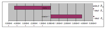Figure 10: Angular momentum of the rotating object in 2 directions, case-1

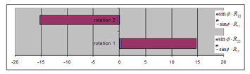Figure 11: Angular momentum of the rotating object in 2 directions, case-2

In Figure 11 for Case-2, the vector’s component of  also appears. In both Case-1 and Case-2, when the speed of the rotation increases from the rotation 1 to the rotation 2, the sign of the angular momentum changes from plus to minus. It means that the direction of the angular momentum reverses when the speed of the rotation of the object changes.

This result suggests a consistency with our previous report on the direction of the spin momentum of gravitational waves [6] shown in Figure 1; however, because gravitational waves are beyond the scope of this extended paper, further discussion on the similarity between the direction of the angular momentum of the antigravity and the direction of the spin momentum of anti-gravitational waves should be postponed to the other research.

Table 5: Intensity of the rotation’s angular momentum, Case-1

	c and  (Rotation 1)	c and  (Rotation 2)
	9.077 (5.072 )	-4.816 (5.931 )
	36.83 (46.33)	-42.94 (45.44)

Table 6: Intensity of the rotation’s angular momentum, Case-2

	c and  (Rotation 1)	c and  (Rotation 2)
	0.2821 (0.2621)	-0.2285 (0.2597)
	14.48 (16.65)	-15.06 (16.69)

3.4. Physical meaning of the results

When the idea of quantum mechanics was developed in the early 20^th century, there was a discussion [11] to select the coordinate system for quantum mechanics from Einstein’s special theory of relativity or his general theory of relativity. He compared two types of the coordinate systems: one was on the flat space-like surface (Figure 12), and another on the curved space-like surface (Figure 13). In each figure, three-dimensional surfaces, S1, S2, S3, S1’ in Figure 12 and S in Figure 13, are placed in four-dimensional time-space, where X₀ is for the time, and X₁, X₂, X₃ for the space. The special theory of relativity is explained in Figure 12, while the general theory of relativity is in Figure 13. Figure 13 represents a three-dimensional curved surface in a four-dimensional space-time, which has the property of being everywhere space-like, and the perpendicular vector to the surface has to be in the light-cone of Figure 13, according to [11].

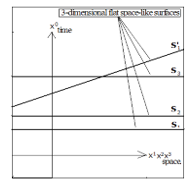Figure 12: Flat space-like surface (remade from [11]

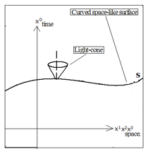Figure 13: Curved space-like surface (remade from [11]

Then it was predicted by [11] that this perpendicular movement to the curved space must have a physical meaning. However, it was found that the curvature tensor could not satisfy the condition for solving the equation of motion in such a perpendicular direction to the curved surface. Henceforward the theory of quantum mechanics was not developed on the curved surface of Figure 13, but on the flat surface of Figure 12.

In our previous research for the conference paper [1], we made a simulation on the energy of the gravitational field, which was the projection on the spherical surface; but, not the movements of the vectors perpendicular to the spherical surface. However, in this extended paper, we also report the result of the simulation of the angular momentum, which is the perpendicular component of the movement of the curved surface. This part challenges the decision to use the flat surface for quantum mechanics in the early 20^th century.

For solving the equation of motion in a three-dimensional curved surface in a four-dimensional space-time, the curvature tensor is needed. But, in our research we used the spherical polar coordinate system as a surrogate of the curved surface so that we could still use the orthogonal transformation of the matrix algebra, which was available originally for the flat space.

The vector components of the spherical surface are the projections of the gravitational energy; and, the movements of these vectors are the movements of the curved surface itself. It looks like Figure 14.

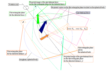Figure 14: The vector projected on the spherical surface

In Figure 14, a flat rectangular plane is put on the surface of an imaginary spherical body. And, inside of the spherical body, there is one arrow that represents the gravitational force. The rotating object, which is not shown in this figure, is assumed to be located in the center of the spherical body. Also one rotation axis is shown in this figure. On this axis, there are two flat rectangular planes: one is for the distorted time, ; and, another is for the distorted distance, . First, the arrow of the gravitational force inside of the imaginary spherical body is projected to each of these two flat planes that are with the signs of  and . Then each of these two arrows is further projected to the flat rectangular plane that touches the surface of the spherical body. Here three vectors of (39) must be on this rectangular plane on the surface, and the calculated coefficients of (38) represent the intensities of the gravitational energy, shown in Figure 8 (Table 3) and Figure 9 (Table 4). If the speed changes in the rotation of the object, the direction of the rotation of the object doesn’t change, but the direction of the projected image of the arrow on the rectangular plane of Figure 14 changes. Here it is noted that we didn’t include  in the simulation for this extended paper.

For simulating the vectors of the angular momentum, we used the cross product of anti-symmetrical vectors as the projection of the momentum vector in the perpendicular direction to the curved surface. It looks like Figure 15. The vectors of (43) are projected on the perpendicular plane with the sign of in this figure. The calculated coefficients of (42) are the intensities of the angular momentum, shown in Figure 10 (Table 5) and Figure 11 (Table 6). If the speed changes in the rotation of the object, the direction of the rotation of the object doesn’t change; but, the direction of the projected image of the arrow changes on the perpendicular plane for  of Figure 15.

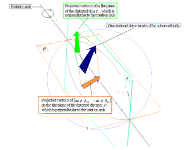Figure 15: The vectors projected on the perpendicular components of the spherical surface

It is noted that we replaced the generally curved surface of Figure 13 by the spherical polar coordinate system as a surrogate for the simulation. And, we mocked the general movement of the curved surface by the rotation of the curved sphere as shown in Figure 15. In Figure 13, the perpendicular movement of the generally curved surface is the movement in the light cone, and it is not necessarily the angular momentum. On the other hand, in Figure 15, the perpendicular movement of the spherical polar coordinate system appears as the angular momentum, only when the system rotates.

4. Conclusions and Recommendations

In this research, we investigated how the intensity and the direction change upon the gravitational energy and the angular momentum when the speed of the rotation of the artificial object changes, using Euler’s rotation matrix by calculating the coefficients of the equation of motion, which is made of the curvature tensor with the component on the curved surface and the perpendicular component to the surface. The result of the simulation shows that the rotating object, in which time and space are nonlinearly distorted by the strong gravity, can produce the antigravity as the projected image on the curved surface, and change the direction of its angular momentum on the projected perpendicular image to the curves surface.

The change of the direction of the angular momentum upon the emerged antigravity implies our previous prediction [6] on the direction of the spin of anti-gravitational waves, in which anti-gravitational waves have the clockwise spin, while gravitational waves have the anti-clockwise spin. However, the conclusion has not been made on this issue because the analysis we described in [6] was made on the flat space, while we made the simulation in the spherical polar coordinate system for this extended paper. In addition, the discussion about gravitational waves is beyond the scope of this extended paper and it should be deferred to the other research; although, the similarity between the antigravity and the anti-gravitational waves may have been implied by the equation of gravitational waves, which is to be derived as the secondary differential of the equation for the gravitational field.

In addition, our simulation has challenged the limit of the general theory of relativity in its application to quantum mechanics, which is: the perpendicular movement to the generally curved surface could not satisfy the condition to solve the equation of motion. Henceforward the curved space was not used for setting quantum mechanics. However, we challenged this limit, by using the spherical polar coordinate system with the tensor algebra that makes the cross product of anti-symmetrical vectors for simulating the projection of the angular momentum in the perpendicular direction to the spherical surface.

In this research, we used the system of spherical polar coordinates as the surrogate of the generally curved surface; however, in the near future, the developed computer technologies must increase the possibility of simulating the generally curved surface of the Einstein’s equations also for solving the equation of motion of quantum particles.

1. Y. Matsuki, P.I. Bidyuk, “Theory and Simulation of Artificial Antigravity,” 2020 IEEE 2nd International Conference on System Analysis Intelligent Computing, 2020, doi: 10.1109/SAIC51296.2020.9239195.
2. Y. Matsuki, P.I. Bidyuk, “Empirical Analysis of Moon’s Gravitational Wave and Earth’s Global Warming,” System Research & Information Technology, N1, 107-118, 2018, doi: 10.20535/SRIT.2308.8893.2018.1.09.
3. Y. Matsuki, P.I. Bidyuk, “Analysis of Moon’s Gravitational-Wave and Earth’s Global Temperature: Influence of Time-Trend and Cyclic Change of Distance from Moon,” System Research & Information Technology, N3, 19-30, 2018, doi: 10.20535/SRIT.2308.8893.2018.3.02.
4. Y. Matsuki, P.I. Bidyuk, “Empirical Investigation on Influence of Moon’s Gravitational-Field to Earth’s Global Temperature,” System Research & Information Technology, N2, 18-24, 2019, doi: 10.20535/SRIT.2308.8893.2019.2.02.
5. Y. Matsuki, P.I. Bidyuk, “Calculating Energy Density and Spin Momentum Density of Moon’s Gravitational-Waves in Rectilinear Coordinates,” System Research & Information Technology, N3, 7-17, 2019, doi: 10.20535/SRIT.2308.8893.2019.3.01.
6. Y. Matsuki, P.I. Bidyuk, “Analysis of Negative Flow of Gravitational Waves,” System Research & Information Technology, N4, 7-18, 2019, doi: 10.20535/SRIT.2308.8893.2019.4.01.
7. Y. Matsuki, P.I. Bidyuk, “Numerical Simulation of Gravitational Waves from a Black Hole, using Curvature Tensors,” System Research & Information Technology, N1, 54-67, 2020, doi: 10.20535/SRIT.2308.8893.2020.1.05.
8. P.A.M. Dirac, “General Theory of Relativity”, New York: Florida University, A Wiley Inter-science Publication, John Wiley & Sons, 1975.
9. H. Goldstein, C.P. Poole, J.L. Safko, Classical Mechanics, 3rd Edition published by Pearson Education. Inc., 2002.
10. A.S. Goldberger, A Course in Econometrics, Harvard University Press, Cambridge, Massachusetts, USA, 1991.
11. P.A.M. Dirac, Lectures on quantum mechanics, originally published by the Belfer Graduate School of Science, Yeshiva University, New York, 1964.

(Click Here)