1. Introduction

This paper is an extension of the work originally presented at IEEE/ASME International Conference on Advanced Intelligent Mechatronics (AIM). IEEE, 2020 [1].

All the environments that we live and work in are designed to be traversed by humans who have a bipedal gait. This makes the bipedal robots advantageous since they would easily adapt to these environments. Bipedal robots can move in discontinuous terrains (ex. stairs) and turn in narrow spots. These and many other reasons have driven researchers to study the bipedal gait as a locomotion method for robots.

There is a variety of methods that researchers can choose to control the gait of a bipedal robot. Using an inverted pendulum model as a template in conjunction with the zero moment point (ZMP) criterion has been used extensively [2], [3]. An up and coming method is obtaining optimal trajectories and inputs through various optimization methods and using them as a reference [4], [5]. Another popular method is to use simple models that can recreate certain fundamental aspects of human or animal gait, as template models for bipedal robots. A template model that is commonly used for this purpose is called the bipedal spring loaded inverted pendulum (SLIP) model [6], [7].

Bipedal SLIP model consists of two complaint legs and a point mass (Figure 2). This model is passive, i.e. there are no external inputs, and its motion is determined by the mechanical parameters and initial conditions. By choosing these carefully, a range of trajectories can be obtained that converge to a limit-cycle. Humans walk in a two phased manner and Bipedal SLIP model can mimic this gait. Human gait is explained with great detail in [8]. These two phases are called single stance phase and double stance phase. In the single stance phase, only one leg is in contact with the ground and the other leg is “swinging”. And in the double stance phase, both feet are on the ground. However, SLIP model has one big assumption that differs substantially from a human gait: in the single stance phase, swing leg is assumed to move instantaneously to the proper

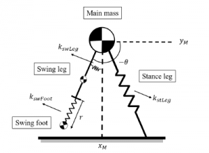
Figure 1: SLIP-SL Model in the single stance phase

touch-down position. This means that when the bipedal SLIP is chosen as the template model for the controller of a bipedal robot, desired trajectories for the swing foot can not be obtained from it. Additional steps are necessary to achieve the swinging motion. [9] proposes a conceptual model where SLIP model is combined with a segmented leg so that the effects of swinging can be studied but reference trajectories and a controller is necessary to achieve the desired motion. In this paper, an extended SLIP model will be proposed so that reference center of mass trajectories and swing foot trajectories can be obtained simultaneously. This model will be called spring loaded inverted pendulum model with swing leg (SLIP-SL) which is shown in Figure 1.

SLIP-SL also has a two-phased gait and in the double stance phase, it is the same as the bipedal SLIP model. The difference is in the single stance phase where the model consists of three massed elements. The model also has three springs to facilitate the movement of these components. SLIP-SL model doesn’t have any inputs, so it keeps the passive nature of the bipedal SLIP. The passive nature necessitates that proper spring parameters and initial conditions are chosen so that feasible trajectories can be realized. In this paper, direct collocation methods [10] were used to conduct simultaneous parameter and trajectory optimization for finding the suitable parameters. Then, a feedback linearization controller is proposed to track the obtained SLIP-SL trajectories with a 5-link fully actuated bipedal robot model. Effectiveness of the proposed controller and SLIP-SL’s ability to be used as a template for walking are investigated through simulation studies.

This paper is organized as follows: Section 2 describes the dynamics of SLIP-SL and the bipedal robot model, Section 3 details the optimization work that is needed for finding feasible SLIP-SL trajectories, Section 4 introduces the proposed feedback linearization controller and in Section 5 simulation results are presented and discussed.

2. Systems and Modeling

This section will begin by introducing the bipedal SLIP model which is followed by the extended SLIP model named SLIP-SL and finally the model for the bipedal robot will be introduced. Explanation of the SLIP model will be brief since there are many works such as [6] that do an excellent job and going in depth on the matter. This paper will focus on the extended model and fully covers it but it is recommended to have a basic knowledge of the SLIP.

2.1        Bipedal SLIP Model

Bipedal SLIP Model can be seen in Figure 2. It consists of a point mass and two massless legs made out of springs. This model can mimic the two phased walking of humans, namely the single and the double stance phase. In the double stance phase, both feet are on the ground and both spring-like legs are pushing the mass. Then, a lift-off event happens where the foot in the back leaves the ground and the model goes into the single stance phase. This phase continues until the touch down event (when the swing foot touches the ground, depending on the angle of attack α and the free length of the spring L₀) at which point it goes back to the double stance phase. This continues in a cycle and walking motion is achieved. The springs are always in contraction and they are always pushing since an actual leg can not pull us towards the ground.

This system is passive so its motion is determined by its parameters such as such as spring stiffness, angle of attack and the initial conditions such as initial the velocity. Different types of gaits can be achieved with this model by changing the parameters and initial conditions so that a stable human-like gait with double peaked ground reaction forces can be achieved. This model has been very popular among researchers because of its simple nature and it has been extensively used to generate reference trajectories for center of mass (CoM) position. However, it has one significant assumption which is that the swing leg is assumed to move instantaneously to the proper position required for touch-down. This is possible since the springs are assumed to be massless. However, this is not the case for actual robots which must perform the swinging motion with actual massed legs so that they can walk. So, when the SLIP model is used as a reference, additional steps are necessary to generate the swing leg motion. Also, since SLIP model ignores the swinging motion, adding it later on might prove to be difficult and will act as a disturbance to the CoM trajectory. That is the advantage of the SLIP-SL model which we will introduce. It is an extension to the SLIP model to include swing leg dynamics in the single stance phase.

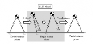
Figure 2: Bipedal SLIP Model

2.2        SLIP-SL model

Spring loaded inverted pendulum model with swing leg (SLIP-SL) can be seen in Figure 1 and its motion throughout a full step is represented in Figure 3. This model also walks in two phases, like its predecessor. In the double stance phase, SLIP-SL and SLIP are identical. What makes SLIP-SL different from the SLIP model is the addition of swing leg dynamics in the single stance phase. In the single stance phase, SLIP-SL consists of 3 massed elements which are the main mass ‘M’, a massed swing leg and a point mass representing the swing foot and 3 springs which are the linear spring that connects ‘M’ to the ground, the torsional spring that is connected between the point mass and the swing leg and the linear spring which connects the swing foot and the swing leg. After the touch-down event, SLIP-SL goes to the double stance phase, the swing elements disappear and the model becomes the same as the SLIP model in the respective phase. SLIP-SL consists of a point mass and two massless springs in the double stance phase.

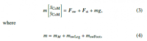
In the single stance phase, equation of motion for the SLIP-SL model can be written as:

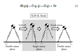
Figure 3: SLIP-SL Model

where q˜ = [x_M,y_M,θ,r]^T are the generalized coordinates, M˜ (q˜) ∈ R^4×4 is an inertia matrix, C˜(q˜, q˙˜) ∈ R⁴ is a Coriolis and centrifugal terms vector, G˜(q˜) ∈ R⁴ is the gravity term, τ˜ ∈ R³ are the resultant forces and torques due to springs and S˜ ∈ R^4×3 is the appropriate mapping matrix for them. The resultant forces can be calculated as:

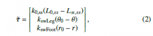
where k₀,_ss, k_swLeg and k_swFoot are the stiffness values for the stance leg spring, the torsional spring at the “hip” and the linear spring connecting the swing foot with the swing leg, respectively and L_0,ss, θ₀ and r₀ are the free positions of those springs where subscript “ss” indicates the single stance phase. L_st is the length of the stance leg. x_M and y_M respectively represent horizontal and vertical positions of the main mass, θ represents the angle of the swing leg with respect to the vertical axis and r represents the distance between the end of the swing leg and swing foot point which are represented in Figure

1. In the double stance phase, dynamics of the SLIP-SL model can be written as:

indicates the total mass of the system, x_CoM and y_CoM are the horizontal and vertical positions of the center of mass and g = [0,−9.81]^T is the gravitational acceleration. Forces generated by the stance and swing leg springs can be calculated as:

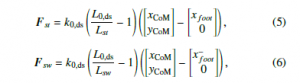
where subscript “ds” indicates the double stance phase. Definitions of x_foot can be seen in Figure 3.

2.3        Bipedal Robot Model

In this part, the dynamics of the 5 linked bipedal robot will be introduced. This model consists of 5 links which are connected to each other with revolute joints and it moves in the sagittal plane. The model is fully actuated and has an ankle torque.

Dynamics of the bipedal robot in the single stance phase can be written as:

where q = [θ₁,θ₂,θ₃,θ₄,θ₅]^T ∈ R⁵ are the generalized coordinates, M(q) ∈ R^5×5 is an inertia matrix, C(q, q˙) ∈ R^5×5 is a Coriolis and centrifugal terms matrix, G(q) ∈ R⁵ is the gravity term, S ∈ R^5×5 is the distribution matrix of actuation torques and u ∈ R⁵ are the input torques. This model can be seen in Figure 4 with the description of generalized coordinates and input torques (indicated with the red arrows).

Like the SLIP-SL model, bipedal robot model also has a two phased walking pattern. In the single stance phase, only one foot is on the ground and other is doing the swinging motion. Single stance phase ends and the system goes into the double stance phase when the swing foot touches the ground.

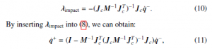
When the swing foot contacts the ground, a collision occurs where the generalized momentum of the system changes discontinuously. This can be modeled by assuming that an impulse force acts on the system to change the velocities while position is kept the same. This can be expressed as:

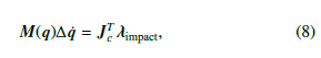
where J_c ∈ R^2×5 is a constraint Jacobian matrix that maps the joint velocities to the swing foot velocity in horizontal and vertical directions. The generalized reaction forces in x and y directions are indicated as λimpact = [λimpactx ,λyimpact]T ∈ R2. Assuming that the impact is inelastic, velocity of the swing foot touching the ground

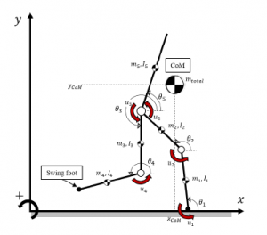
Figure 4: 5 link fully actuated robot model will become zero after the impact which can be written as:

which are the generalized velocities just after the impact. At the moment of impact, definitions of the legs are also switched (swing leg becomes the stance leg and vice versa).

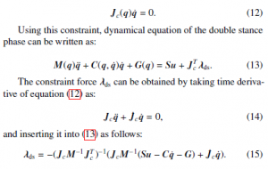
The system is now in the double stance phase where both feet are in contact with the ground. To model this, a constraint force λ_ds = [^λ_ds^x ,λ^y_ds]^T ∈ R² is added to keep the swing foot on the ground. In the vertical direction, this constraint force can only push the robot (λ^y_ds > 0). With the non-slip assumption, double stance phase dynamics can be modeled by introducing the following constraint:

3. Direct Collocation Optimization

In this section, the optimization conducted to find periodic trajectories for SLIP-SL will be described. SLIP-SL is a passive model which means its gait solely depends on its mechanical parameters and initial conditions. In order to find the proper value, Direct Collocation Methods [10] were used in this study. These methods tackle the trajectory optimization problem by discretizing and converting it into a form which can be handled by nonlinear programming (NLP) solvers. There are many commercially available NLP solvers and in this study OpenOCL [11] will be used which can handle the multi-phase and simultaneous trajectory and parameter optimization problem. Finding the global minimum is not guaranteed when using the direct collocation methods. Global minimum is not easily found in a nonlinear problem with constraints such as 16. The advantage of direct collocation over other optimization methods such as genetic algorithms or learning based algorithms is that dynamics of the system can be embedded as constraints to the optimization problem painlessly.

The optimization can be formulated as:

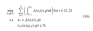
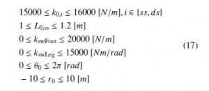
where t ∈ [0,T_i] is the time, T_i is the end time of the respective phase, x_i(t) is the state trajectory, p are the parameters, J_i(x, p) are the path cost functions, f_i(x, p) are the system dynamics (described in Section 2.2) and r_i,k(x_i, p) are the grid-constraints. i = 1 represents the single stance phase and i = 2 represents the double stance phase for SLIP-SL (T₁ is when the touch-down happens at the end of “ss” and T₂ is when the lift-off happens at the end of “ds”). In this paper, the Cost of Transport (CoT) [6] and a cost function to keep the swing foot low was used. CoT is an indicator of the walking efficiency.

Path, boundary and stage transition constraints are needed so that the solver can find feasible walking trajectories. Path constraints are:

• Bounds were set for the parameters to be optimized:

• Stance leg spring in the single stance phase and both legs’ springs in the double stance phase are always under contraction: L_st,ss ≤ L₀,ss, L_st,ds ≤ L₀,ds, L_sw,ds ≤ L₀,ds
• Constraining the vertical position of CoM: 0 [m] ≤ y_CoM ≤ 0.85 [m]
• Swing foot is always above the ground during the single stance phase: y_swFoot ≥ 0
• Elliptic virtual obstacle must be avoided by the swing foot during the single stance phase:

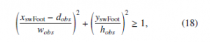
where d_obs = x_swFoot = 0 [m] is the horizontal position of the ellipse obstacle, w_obs = 0.2 [m] and h_obs = 0.04 [m] are width and height of the ellipse.

• Swing foot vertical velocity must be greater or equal to zero: x˙_swFoot ≥ 0
• Vertical acceleration of CoM should be negative in the single stance phase so that system doesn’t try to lift the CoM up when there is only one leg on the ground: y¨_CoM,ss ≤ 0 [m/s²]

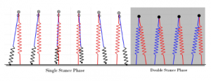
Figure 5: Snapshots of SLIP-SL’s one step where gray dot in the single stance phase indicates the position of the point mass ‘M’ and the circle indicates the position of CoM Boundary constraints:

• Swing foot starts on the ground from a stationary position in the beginning of the single stance phase and touches the ground at the end of the single stance phase: y_swFoot(0) = 0, x˙swFoot(0) = 0, ˙yswFoot(0) = 0, yswFoot(T1) = 0
• Initial step length and the final step length should be same

(for cyclic walking): xfoot − xfoot− = xfoot+ − xfoot

• The initial position of the main mass relative to the stance foot should be the same as the final one (for cyclic walking): xstFoot,0 − xM(0) = xstFoot(T2) − xM(T2)
• Constraints for cyclic walking: y_CoM(0) = y_CoM(T₂), x˙CoM(0) = x˙CoM(T2), ˙yCoM(0) = y˙CoM(T2)
• At the stage transition, CoM position and velocity were constrained to be continuous.
• At the end of the double stance phase, swing leg should be ready to lift off, i.e. swing leg spring should be at its free length: Lsw,ds(T2) = L0,ds

Parameters to be optimized are spring stiffness values k_0,ss, k_0,ds, k_swFoot, k_swLeg, their respective free positions L₀,_ss, L₀,_ds, r₀,θ₀ and the initial conditions.

The optimization was conducted on MATLAB 2019b software by using 10 collocation points for each stage. Resulting spring parameters can be seen in Figure 6 for various trajectories and a snapshot of SLIP-SL’s one step can be seen in Figure 5 for a sample trajectory. Trajectory ‘A’ from Figure 6 will be used as the reference in Section 5 where the step size was also constrained to 0.25 [m] to avoid large ankle torques. The constant mechanical parameters of SLIP-SL are given in Table 1.

Table 1: SLIP-SL’s constant mechanical parameters

m_M : 70 [kg]              m_swLeg : 7 [kg] mswFoot : 3 [kg]             Lthigh : 0.7 [m]

           IswLeg = mswLegl_thigh²    /12 [kg · m²] IswFoot = mswFootL_thigh²

4. Feedback Linearization Control

In this section, the proposed controller will be introduced so that 5 linked bipedal robot model can track the reference SLIP-SL trajectories. The controller uses the feedback linearization notion, in a similar manner to [12] where a total energy control approach was used with the bipedal SLIP model. However, in this paper, a trajectory tracking approach will be used.

4.1        Single Stance Phase

For the control of the robot in the single stance phase, there are three main tasks: tracking CoM trajectory x_G ∈ R², tracking swing foot trajectory ξ ∈ R², controlling the trunk orientation θ₅ ∈ R. The velocities related to these tasks can be calculated as:

where x˙_t,ss = [x˙_G,ξ˙,θ˙₅]^T is the velocity in the task space where subscript “ss” indicates the single stance phase and J_t,ss(q) = [J_G, J_ξ, J_θ5]^T are the combination of Jacobian matrices. J_G maps generalized velocities to the velocity of the center of mass, J_ξ maps generalized velocities to swing foot velocities and J_θ5 maps generalized velocity to the trunk’s angular velocity. By taking the time derivative of Equation (19) and inserting the obtained q¨ into Equation (7) we can get:

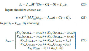
where K_P and K_D are the proportional and derivative gains for the controller and θ_5,des is the desired trunk angle, desired trajectories can be tracked. Desired trajectories will be chosen as the SLIP-SL trajectories that were obtained in Section 3. In this study, the desired trunk angle was chosen as θ_5,des = π [rad].

4.2        Double Stance Phase

During the double stance phase, swing foot remains on the ground which means there is one less task to be carried out. This means that some modifications should be made to the single stance phase controller so that it can be used in the double stance phase. The task space for the double stance phase then becomes:

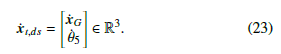
This reduction in dimension of the task space is somewhat problematic since we need to determine 5 separate inputs but the dimension of x˙_t,ds is 3 which means there is more than one correct way to allocate the inputs. To calculate the proper inputs, the following equation can be used:

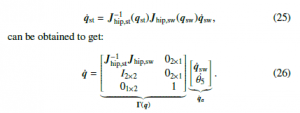
where J_{hip, i}(q_i) is the jacobian matrix that maps the corresponding legs angular velocities, q˙_st = [θ˙₁,θ˙₂]^T and q˙_sw = [θ˙₃,θ˙₄]^T, to the velocity of the hip. This holds since both foot are on the ground during the double stance phase. From equation (24),

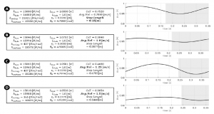
Figure 6: Optimization results for various SLIP-SL trajectories. For the trajectory A, step length was constrained to 0.25 [m] to get better ankle torques and this trajectory is the one that was used as reference in Section 4. For B, C and D trajectories, average velocity constraints were added. In this figure, resulting mechanical parameters, costs of transport and step length are given as well as the SLIP-SL’s y_CoM trajectory. In the plots on the right, gray background means that the SLIP-SL is in double stance phase.

After taking the time derivative of (26), then substituting the            q¨ and q˙ terms from (26) into (7) and multiplying with Γ^T from left, following can be obtained:

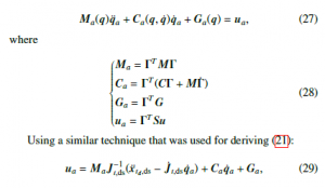
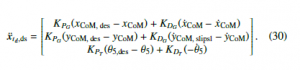
can be found where x¨_td,ds should be chosen as:

However, only u_a ∈ R³ can be obtained in this way which only has dimension 3. What we need to control the robot is u ∈ R⁵. One way to calculate u is by using the relation u_a = Γ^TSu given in (28) as:

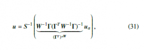
where (Γ^T)^+W is the weighted matrix inverse operation. W ∈ R^5×5 matrix can be used to penalize high input torques such as the ankle torque but we selected it as identity matrix for this paper.

Controllers for the single and double stance phases are thus derived. Another important aspect of the controller in tracking the SLIP-SL trajectories is the switching of phases at the correct moments. When the biped robot is in the double stance phase and the tracked trajectory goes into single stance phase, controller switches to the single stance phase controller and commands the robot to lift its foot so it too can switch to the proper phase.

5. Simulation Results and Discussion

In the following simulation study, the designed controller’s ability to track the reference SLIP-SL trajectories and the suitability of the SLIP-SL as a template model for walking will be tested. Table 3 shows the mechanical parameters of the 5 link robot and Table 2 shows the chosen gain values for the controller and the torque limits on the motors were set at 200 [Nm]. Gain values are chosen with the help of a particle swarm optimization algorithm (PSO) [13]. We were able to find controller parameters that resulted in stable gaits easily by hand-tuning but with the help of PSO we were able get results with better walking efficiency.

Table 2: Control Parameters

KPG : 54	KDG : 9
KPsw : 82	KDsw : 8
KPT : 36	KDT : 4

The simulations were implemented in MATLAB 2020b’s Simulink environment with ode45 solver and variable step settings (absolute tolerance was set to 1e-8).

Figure 7 shows the resulting CoM trajectory and trunk orientation the controlled system when the proposed controller is used. Figure 8 shows the swing foot trajectories for the same system. It can be seen that the proposed controller does a good job in tracking the reference trajectories of the SLIP-SL template, which were obtained in Section 3. The reference SLIP-SL trajectories for the swing foot would not be available if a template such as the popular SLIP was used.

Table 3: 5 Link Model Parameters

l₁ = l₄ : 0.48 [m]           l₂ = l₃ : 0.48 [m]     l₅ : 0.48 [m] m₁ = m₄ : 5 [kg]                m₂ = m₃ : 5 [kg]     m₅ : 60 [kg]

I_i = m_il_i²/12 [kg · m²], i = 1,2,3,4,5

It can be seen in Table 2 that relatively low gains were chosen for this study. Tracking performance can be increased by using larger gains but since this model is fully actuated and has an ankle torque, zero moment point (ZMP) condition must also be checked. ZMP criterion states that if the center of pressure moves to the toe (or to the “outside” of the foot), foot would rotate and system would be under actuated [14]. For this trajectory, center of pressure stays within a 30 [cm] foot.

Figure 9 shows snapshots of one step of the 5 link models gait. to check the stability of the gait, Poincare map approach was consid-´ ered [12]. The dimensions of the Poincare map were selected as the´ θ_P = atan2(y˙_CoM, x˙_CoM), y_CoM and total energy of the 5 link model E at the vertical leg orientation (VLO). VLO happens when CoM of the 5 link model is at the same horizontal position as the stance foot. VLO was chosen as the Poincare section because the horizontal po-´ sition doesn’t need to be considered at this point. Poincare stability´ criterion indicates that if the return map converges to a fixed point, a hybrid system with impact effects can be considered periodic [12]. Poincare Map for the controlled 5 link model is shown in Figure 10. It can be seen that the gait converges to a stable point in the section after a couple of steps which indicates stability.

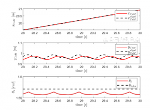
Figure 7: Trajectory tracking results for CoM horizontal position, vertical position and trunk orientation

The CoT value for the reference SLIP-SL trajectory was 0.7520 and this value is 0.7745 for the controlled 5 link robot. Also, the average velocity of the SLIP-SL trajectory was 0.7080 [m/s] and this value was 0.6974 [m/s] for the controlled system. These values being very similar between the reference and the controlled model also indicates the validity of the proposed controller. Cost of transport being slightly higher is expected because the 5 linked model needs to keep its body upright but SLIP-SL doesn’t have this issue.

In this paper, it was also shown that by using direct collocation optimization, various SLIP-SL trajectories can be obtained (Figure 6) that resemble the walking gait. Cost of transport tended to decrease when the average velocity of the gait was increased and step length was not constrained but this kind of trajectories can be more demanding on the inputs and they sometimes resulted in large ankle torques which was troubling for the ZMP criterion. Also stiffness of the legs were limited to 15000 [Nm] ≤ k_0,i ≤ 16000 [Nm], i ∈ {ds, ss} to keep the CoM height within a certain range.

This stiffness limits was chosen to have a similar height trends with [12] and [6] where k₀ was 15696 [Nm]. It can be seen that k_0,ss , k_0,ds for the given trajectories but it was possible to find feasible trajectories with k₀,_ss = k₀,_ds, even with k₀,_ss = k₀,_ds =

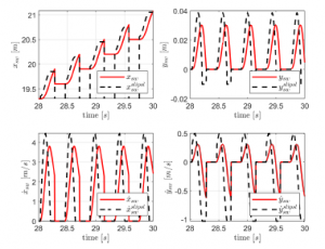
Figure 8: Trajectory tracking results for the swing foot

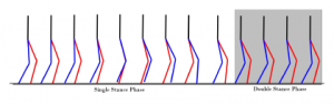
Figure 9: Snapshots from a step of the 5 Link model

15696 [Nm] but this doesn’t really mean that linear leg springs were the same in single and double stance phase since L_0,ss , L_0,ds. The free length of the springs in the double stance phase was set to 1 [m] to be the same with [12] but L_0,ss needs to be larger than this value to keep the CoM high enough. If L_0,ss was 1.0 [m], CoM would sag further than desired range in the single stance phase.

6. Conclusion

In this paper, a template model called SLIP-SL was proposed which is an extension to the popular SLIP model. SLIP model can generate the reference CoM trajectories that can mimic the two-phased walking but it doesn’t have the swing leg dynamics. Thus, when this template model is used, additional steps are necessary for obtaining the swing foot trajectory so that the actual robot can be controlled. Since the swinging motion is a huge part of the walking gait that needs to be taken into account, SLIP-SL adds this dynamics while keeping the passiveness of the SLIP model.

Since the SLIP-SL is passive, proper mechanical parameters and initial conditions needs to be determined to get feasible walking trajectories. It was demonstrated that direct collocation methods can be used to find the proper parameters for the passive SLIP-SL model. This step was crucial since there are many parameters that needs to be decided and other more exhaustive search methods might not work. It was shown that a variety of trajectories with different average velocities, CoM behaviors etc. can be obtained using the same basic principles. Then, a controller was introduced to track the

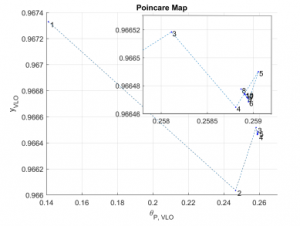
Figure 10: 2D section of the Poincare Map where the numbers indicate the step´ number (zoomed in version is shown in the right upper corner of the figure)

obtained reference trajectories and it was shown that it can satisfactorily track the reference SLIP-SL trajectories to reach a stable gait while also satisfying the ZMP criterion. These results also confirmed that SLIP-SL can be used as a template model for walking robots.

In the future, we would like to introduce robustness to this passive system by making the springs variable ones and controlling them to reject disturbances. Another area we would like to explore is achieving a variable speed gait with the bipedal model. We want to achieve this by smoothly switching between different reference SLIP-SL trajectories.

1. M. M. Pelit, J. Chang, R. Takano, M. Yamakita, “Bipedal Walking Based on Improved Spring Loaded Inverted Pendulum Model with Swing Leg (SLIP-SL),” in 2020 IEEE/ASME International Conference on Advanced Intelligent Mechatronics (AIM), 72–77, IEEE, 2020, doi:10.1109/aim43001.2020.9158883.
2. S. Kajita, F. Kanehiro, K. Kaneko, K. Fujiwara, K. Harada, K. Yokoi, H. Hirukawa, “Biped walking pattern generation by using preview control of the zero-moment point,” in 2003 IEEE International Conference on Robotics and Automation (Cat. No. 03CH37422), volume 2, 1620–1626, IEEE, 2003, doi:10.1109/robot.2003.1241826.
3. R. Takano, M. Yamakita, “Sequential-contact bipedal running based on SLIP model through zero moment point control,” in 2017 IEEE International Conference on Advanced Intelligent Mechatronics (AIM), 1477–1482, IEEE, 2017, doi:10.1109/aim.2017.8014227.
4. H. Yano, J. Chang, R. Takano, M. Yamakita, “Simultaneous Optimization of Trajectory and Parameter for Biped Robot with Series Elastic Actuators,” IFAC-PapersOnLine, 52(22), 7–12, 2019, doi:10.1016/j.ifacol.2019.11.039.
5. A. Patel, S. L. Shield, S. Kazi, A. M. Johnson, L. T. Biegler, “Contact-implicit trajectory optimization using orthogonal collocation,” IEEE Robotics and Automation Letters, 4(2), 2242–2249, 2019, doi:10.1109/lra.2019.2900840.
6. J. Rummel, Y. Blum, A. Seyfarth, “Robust and efficient walking with spring-like legs,” Bioinspiration & biomimetics, 5(4), 046004, 2010, doi: 10.1088/1748-3182/5/4/046004.
7. H. Geyer, A. Seyfarth, R. Blickhan, “Compliant leg behavior explains basic dynamics of walking and running,” Proceedings of the Royal Society B: Biological Sciences, 273(1603), 2861–2867, 2006, doi:10.1098/rspb.2006.3637.
8. J. S. Park, C. M. Lee, S.-M. Koo, C. H. Kim, “Gait phase detection using force sensing resistors,” IEEE Sensors Journal, 20(12), 6516–6523, 2020, doi:10.1109/jsen.2020.2975790.
9. M. A. Sharbafi, A. M. N. Rashty, C. Rode, A. Seyfarth, “Reconstruction of human swing leg motion with passive biarticular muscle models,” Human movement science, 52, 96–107, 2017, doi:10.1016/j.humov.2017.01.008.
10. M. Kelly, “An introduction to trajectory optimization: How to do your own direct collocation,” SIAM Review, 59(4), 849–904, 2017, doi:10.1137/ 16m1062569.
11. J. Koenemann, G. Licitra, M. Alp, M. Diehl, “OpenOCL–Open Optimal Control Library,” 2017, doi:10.1137/16m1062569.
12. G. Garofalo, C. Ott, A. Albu-Scha¨ffer, “Walking control of fully actuated robots based on the bipedal slip model,” in 2012 IEEE International Conference on Robotics and Automation, 1456–1463, IEEE, 2012, doi: 10.1109/icra.2012.6225272.
13. J. Kennedy, R. Eberhart, “Particle swarm optimization,” in Proceedings of ICNN’95-international conference on neural networks, volume 4, 1942–1948, IEEE, 1995, doi:10.5772/6754.
14. E. R. Westervelt, J. W. Grizzle, C. Chevallereau, J. H. Choi, B. Morris, Feed-back control of dynamic bipedal robot locomotion, CRC press, 2018, doi: 10.1201/9781420053739.

(Click Here)