1. Introduction

This paper is an extension of work originally presented at the 24th European Conference on Circuit Theory and Design, ECCTD 2020 [1] and this is refinement of work where we proposed simulation tool for analyzing ensembles of oscillators.

Studying the collective behavior of coupled oscillators is fundamental problem that has wide application in nature, science, and technology. Simulation of large networks of coupled oscillators is actual multidisciplinary problem due to high demand in various research areas of including biology, chemistry, physics, electronics etc. [2].

The relevance of this issue has been constantly increasing recently due to the growing interest in the study of oscillatory neural networks [3, 4], to the problem of mutual injection locking of oscillators under parasitic couplings in integrated circuits [5], and to various other applications.

The ensemble of physical oscillators is described by system of ordinary differential equations (ODE). Respectively, the analysis of the ensemble can be performed by numerical methods for ODE solving. This approach is effective for an ensemble with small number of simple oscillators [6]. Direct ODE solving of large oscillator ensembles requires too high computational effort. Therefore, simplified models are required for effective simulation of large oscillator systems [7].

The simplification techniques assume that the coupling strength between the oscillators is rather weak [8, 9]. In this case the coupled oscillator waveform can be considered to coincide with the waveform of this oscillator in free running mode. Then the set of system variables includes only the phases of the oscillators.

The most widespread simplified model is the Kuramoto model (KM) [4, 9, 10] represented by ODE system with respect to phase variables. Kuramoto model describes each oscillator with a single phase variable. The oscillatory interconnections are described in Kuramoto model by 2π-periodic coupling functions.

The standard mathematical packages are usually used for the KM numerical solving. Most often Matlab software [11] is applied (see, for example, [12, 13]). Also, Python codes can be used for solving KM ODE system [14, 15].

However, using standard software packages leads in practice to some difficulties and does not provide effective simulation of an ensemble of oscillators in many applied cases. The user needs to think through the names of variables, repeatedly include the same operators in the code and describe the necessary operations for each specific task. This increases the amount of data preparation, takes a lot of time and leads to additional user errors.

For this reason, the development of universal approach and software tool to improve numerical efficiency of Kuramoto model applications and provide convenient analysis of the simulation results is the actual problem of simulation of ensemble of physical oscillators.

The above limitations are the motivation for the development of new numerical approaches that significantly increase the usability of applied tools.

The paper [16] is devoted to this topic. The paper is directed to reduce the arisen difficulties in process of the numerical solution while KM application. The approach [16] is based on representing the KM in the form of the state equations for an equivalent electrical circuit and applying an electrical simulation tool to this circuit. The obtained circuit simulation results are numerically equal to the results of KM simulation.

However, the implementation of the approach presented [16] has the following disadvantages:

• an equivalent circuit is constructed under the wave digital concept [17] which is run on digital signal processors and is not suitable for standard circuit simulators;
• coupling functions in KM can only be represented by sinusoids with the same amplitude, arbitrary functions are not allowed;
• considered sinusoidal coupling functions cannot include phase delay that leads to the impossibility to analyze some important types of coupled oscillators.
• The contribution of the presented paper is connected with new approach that allows to eliminate the limitations of [16]. We propose the following principles for constructing KM equivalent circuit:
• the equivalent circuit should be suitable to analyze by means of standard circuit simulators. Such a circuit consists of standard electrical components which can be described by input netlist;
• coupling functions of arbitrary 2?-periodic form can be considered in KM and specified by truncated Fourier series with the given harmonics amplitudes and phases;
• special-purpose technique to generate the equivalent circuit netlist should be applied.

In comparison with paper [1] the contribution involves additional simulation example to illustrate capabilities of the developed approach for analyzing oscillator ensembles.

The rest of the paper is organized as follows. Section 2 describes the known mathematical forms of the KM equations. Section 3 explains the forming the equivalent circuit for a given KM. Section 4 outlines the principles for the netlist generation procedure. Numerical experiments are presented in Section 5.

2. Kuramoto Model

2.1. Basic Model Equations

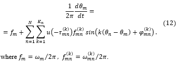
KM defines the behavior of a system of N weakly coupled oscillators. Each oscillator is characterized by its natural frequency (fundamental)  and the time-varying instantaneous phase . In its simplest form, corresponding to the initial Kuramoto proposal (1) KM is represented as an ODE system [18, 19]:

here K is the coupling strength assumed to be the same for all couplings. This form made it possible to obtain estimates of the behavior of the synchronized ensemble of oscillators. However, the assumption about the same couplings is not met in most cases, so more general form of KM was proposed [20, 21]

here  is the individual coupling strength between m-th and n-th oscillators. Form (2) of KM is more flexible tool to represent real sets of coupled oscillators.

The natural extension of KM also considers the external periodic force [22, 23] as the excitation with a given phase  applied to internal oscillators. In such case the Right-Hand Side of m-th equation (2) is supplemented by external coupling functions of the form  .

In the simplest case when one oscillator is excited by a single stimulus, the KM equation has the form:

The phase of the periodic excitation is  where  is the excitation frequency that in the synchronized mode coincides with the oscillator frequency. The oscillator phase is  where φ is the initial phase of the synchronized oscillator. After substituting expressions for phases  into (3) we obtain the algebraic equation with respect to ϑ and the condition of its solution existence defining the locking range of the oscillator

In general case the locking range  of m-th oscillator under the excitation by n-th oscillator is equal to the coupling factor .

System (2) with antisymmetric sinusoidal coupling functions always results in a synchronized behavior for a set of identical oscillators. However, starting from [24], it was found that some dynamical systems of identical oscillators can demonstrate unsynchronized states with quasiperiodic oscillations. Such states, defined as  chimeras [25, 26], can be represented by KMs with additional phase shifts in sinusoidal arguments. Using notation (5), we can write:

that can also be presented as the sum of sines and cosines due to .

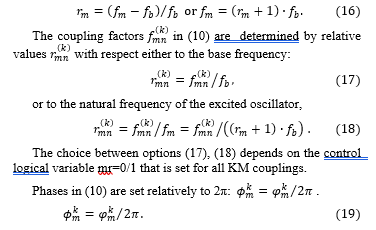
KM in the form (6) does not capture some of the effects inherent in coupled oscillators. E.g., superharmonic synchronization [27] of m-th oscillator under the excitation by k-th harmonic of n-th oscillator cannot be taken into account.  Thus, more complicated coupling functions are needed, and the most general form of KM was defined as [10, 22]

Here  are 2π-periodic coupling functions that are often approximated to desired accuracy using truncated Fourier series with sufficiently large number of terms:

Constant terms in the Fourier series (5) are zeroes ( ) due to the compensation of nonzero terms by the change of fundamentals  in (1). Similarly, diagonal entries are also assumed to be  for all k.

Under notations (5) one can represent (8) as

Here  is equal to the locking range of superharmonic synchronization [13] of m-th oscillator under the excitation by k-th harmonic of n-th oscillator.

2.2.  Modified Model Equations

To enhance the user-friendliness when simulating coupled oscillators, we have made some modifications to the KM (9).

Couplings activation moments were included in the model assuming all couplings were initially disabled.

The activation moment is defined by adding to the coupling function time-dependent multiplier  were u(t) is the unit step function,   is the coupling activation moment. Then coupling function from KM (6) has the form:

For the coupling functions defined by Fourier series (8), (9) we indicate the activation moment   for each k-th Fourier term.

Main results of KM simulations are presented by oscillator phases . However, the phase waveforms are often inconvenient for analyzing the simulation results due to include a linear component. More user-friendly data is represented by instantaneous frequency waveforms, that indicate the synchronization mode by their constant values. The instantaneous frequency in angular ( ) or regular ( ) forms is determined as following:

Note that the angular form of the instantaneous frequency  (7) is used in any KM form (1), (2), (6) and (9). This also corresponds to the Right-Hand Side of KM. But usually the user needs to analyze the frequency in the regular form , so to avoid superfluous transforms one can convert KM to a form with respect to regular frequencies by dividing it by 2π. Then KM (9) is represented as

3. Representation of Kuramoto Model by Equivalent Electrical Circuit

The behavior of the oscillator ensemble can be obtained by the simulation of the electrical circuit if state equations of the circuit coincide with the KM ODE system (12) of the ensemble. Thus, we proposed the following structure of the equivalent circuit.

Each m-th oscillator from KM corresponds to the node in the equivalent circuit with the same index m. The voltage of the node is equal to the phase of KM (12): .

The devices connected in parallel to m-th node include:

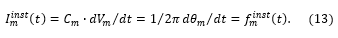
1. Capacitor C_m=1/(2π) representing the phase differentiation in the left-hand side of (12). The capacitor current is numerically equal to the instantaneous frequency of m-th oscillator:
2. Independent current source numerically equal to the fundamental of m-th oscillator
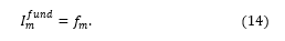3. Nonlinear current sources correspond to Fourier terms in the Right-Hand Side of (9). Each source represents k-th Fourier harmonic of a coupling function from m-th to n-th oscillator:

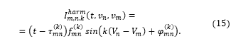here parameters  are defined in KM (12).

One can see that Kirchhoff Current Law (KCL) equations for the equivalent circuit with M nodes corresponding to all oscillators of KM represent the same ODE system as the initial KM:

• the KCL equation for the node of m-th capacitor coincides with m-th equation of KM (12),
• the voltage (V) of m-th node is numerically equal to the instantaneous phase (rad) of m-th oscillator,
• the current (A) through m-th capacitor is numerically equal to the instantaneous frequency (Hz) of m-th oscillator due to (11).

Note that m-th node in the equivalent circuit (13-15) is floating due to the capacitor connection to the current sources. Hence the initial capacitor voltage equal to the initial oscillator phase should be defined to provide transient simulation.

The example in Figure 1 represents the equivalent circuit for KM of the pair of coupled oscillators.

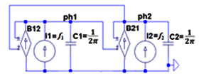Figure 1: The equivalent circuit for KM of the pair of coupled oscillators.

Input netlist of the circuit in Figure 1 for oscillators’ fundamentals f₁=100Hz, f₂=102Hz and couplings parameters, f₁₂=f₂₁=1Hz, τ₁₂=1sec., τ₂₁=5sec. has the form:

Input netlist for KM of the pair of coupled oscillators.
.params inv2pi=0.5/pi    *parameter to define constant 1/2π * oscillators (13) C1   0   ph1  {1/2π} C2   0   ph2  {1/2π} * fundamentals (14) I1   ph1  0  100 I2   ph2  0  102 * couplings  (15) B12 ph1 0 I = 1*sin(v(ph2,ph1))*u(time – 1) B21 ph1 0 I = 1*sin(v(ph1,ph2))*u(time – 5) * initial phases of oscillators .IC .IC
.end

After processing the netlist by LTspice circuit simulator [28] one can obtain instantaneous frequencies of oscillators as current waveforms of capacitors C1 and C2 (13). Examples of the waveforms I(C1), I(C2) are presented in Figure 2.

The waveforms in Figure 2a are obtained for parameters given in the presented netlist. While both couplings at t < 1sec are disabled the oscillators produce their natural frequencies f₁=100Hz and f₂=102Hz.  At t=1sec coupling 1-2 is activated but the coupling factor f₁₂=1Hz is insufficient (|f₁– f₂| =2 > f₁₂) to provide synchronization  of the oscillator #2 by the oscillator #1. So, beats appear in the instantaneous frequency waveform at 1 < t < 5sec. After the activation of both couplings at t > 5sec the oscillators are mutually synchronized with common frequency 101Hz.

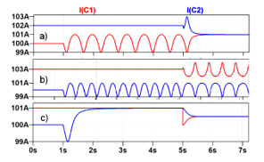Figure 2: Simulated waveforms of instantaneous frequencies of capacitances currents obtained for f1=100Hz and a) f2=102Hz, b) f2=103Hz, c) f2=101Hz

Figure 2b demonstrates simulation results for an increased value of the second fundamental to f₂ = 103Hz. results for an increased value of the second fundamental to f₂ = 103Hz. The discrepancy of fundamentals is too large (|f₁–f₂| = 3Hz) to provide synchronization even under the activation of both couplings.

The decrease of the second fundamental to f₂=101Hz ((|f₁– f₂| =1Hz) leads to waveforms in Figure 2c with synchronization under both unidirectional and bidirectional couplings.

4. Automatic Forming of Input netlist by Matlab Description of Kuramoto Model

For the convenience of forming a Input netlist of an equivalent electrical circuit, we introduce the naming rules for nodes and components of the circuit that is shown in Table 1.

Table 1: Netlist names corresponding to m-th oscillator.

m-th circuit components (KM variable)	Notation	Netlist name
m-th node (m-th oscillator)	m	phm
Node  voltage (oscillator phase)	vm	v(phm)
m-th capacitor	Cm	Cm
Capacitor current (instantaneous frequency)		I(Cm)
m-th DC current source (natural frequency)		Im
Behavioral current source (coupling harmonic) k – harmonic index, m,n – oscillators indexes		Bm_n_k

In accordance with Table 1 netlist  fragment corresponding to m-th oscillator is presented  by the following types of lines:

Cm             0     phm      {1/2π};   differentiation operator

Im            phm     0          f_m;          natural frequency

…………………………………………

Bm_n_k   phm   0                   k-th harmonic of mn coupling

…………………………………………..

…………………………………………..

.IC  ;            initial phase of m-th oscillator

One can see from this fragment that the netlist of the equivalent circuit contains significant amount of duplicate or redundant text data because the same oscillator indexes can be repeated in many component names. For example, the oscillator index m is included in the name of the node representing the oscillator phase and in the name of each component connected to the node.

Redundancy increases for the netlists with many Fourier harmonics (Bm_n_k). In this case  the same indexes of oscillators must be presented in each behavioral source (Bm_n_k) both as the part of its name and names of reference nodal voltages v(phn).

To eliminate the redundancy of the input data, we propose to generate the Input netlist using the procedure based on the description of interacting oscillators in compact form without data duplication. The form is convenient for filling out by the user.

When developing the procedure, we firstly changed the set of primary parameters in favor of relative values. Considering that KM is applicable to the ensemble of oscillators with close natural frequencies one can introduce the “base frequency” parameter , which is close to average fundamentals of all oscillators.

Individual natural frequencies are set by defining its relative deviations ( ) from the base frequency:

The procedure to generate an Input netlist is developed using Matlab software [7], so parameters (13) – (15) are grouped in the Matlab data types that include:

1. Simple numeric variables:

 – fb – basic frequency.

 – mr – type of relative parameter.

 – Tsim – simulation time.

2. Cell array osc that contains oscillators’ parameters. Each array element contains parameters of one (m-th) oscillator:

• the relative deviations of natural frequency r_m (16);
• the initial phase θ_m(0).

The oscillator parameters are set by assigning them to the array element with the oscillator index, e.g.

osc{n1} =[ r_n1   θ_n1(0)];

osc{n2}=[ r_n2];

……

osc{nL}=[ r_nL θ_nL (0)];

Oscillator indices (n1, n2, …nL) are arbitrary non-repeating integers. The value of zero initial phase can be  omitted (see n2).

3. Cell matrix coup with parameters of couplings. Each matrix entry (m, n) defines cell array of parameters of harmonics (15) for given indexes of excited (m) and exciting (n) oscillators. The sequential number of the parameter vector presents the harmonic index k and components of the vector define coupling factor, phase shift and switching moment of the harmonic. Thus, the coupling function (m, n) with k harmonics is represented as matrix entry with parameters of all harmonics:

coup{m,n}={[ ][ ] … [ ] };

For example, the pair of coupled harmonic oscillators in Figure 1 is defined by the following description:

fb=100;

osc{1}=[0];

osc{2}=[0.06];

coup{1,2}={[0.01 0  1]};

coup{2,1}={[0.01 0  5]};

One can see that this description is more compact than presented above Input netlist of the equivalent circuit in Figure 1. More essential reducing of the size of input data can be achieved for KM containing many coupling functions with large number of Fourier harmonics.

Thus, to simulate the oscillator ensemble defined by the given KM one should perform the following operations:

• form Matlab description of the KM by filling-in cell array osc with parameters of oscillators and filling-in cell matrix coup with parameters of couplings;
• generate Input netlist by applying the developed procedure to the formed KM description;
• apply standard circuit simulator to the generated netlist;
• analyze time-domain dependences of phases and frequencies by applying the simulator waveform viewer to the corresponding nodal voltages and capacitances currents.

5. Numerical Examples

Here we present two numerical examples that illustrate the application of the developed approach to the analysis of ensembles of oscillators. To simulate the generated equivalent circuit, the LTspice circuit simulator [28] was used.

The first example presents 8 ensembles of 9 oscillators with natural frequencies evenly distributed in the interval [98 – 102] Hz:

The oscillators are sequentially coupled in forward direction and have one or two reverse couplings forming different versions of closed sequence that are shown in Figure 3.a1-a8. The figure 3aN represents the  version with the index N of the intermediate oscillator between reverse couplings (Figure 3a1 is the version  with one coupling).

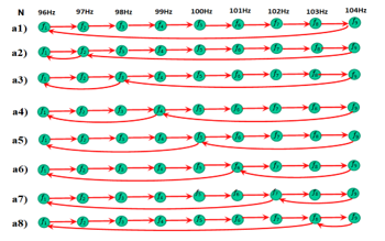Figure 3: Series of oscillators 1-8 with reverse couplings through N-th oscillator:  aN), N=1…8.

All couplings in each ensemble a1-a8 are defined by sine functions (2) with the same coupling factor  = ρ (for all m, n).

The aim of the experiments is to determine for each version the value of the common coupling factor providing the ensemble synchronization – ρ_synch and to compare obtained values for different versions. To obtain the results  the ensembles in Figure a1-a8 must be simulated for a range of overall coupling factors.

To perform the simulation the developed procedure was applied. As an example we present below Matlab descriptions of KM for a1, a5 and corresponding simulation results.

% Matlab description for KM a1

fb = 100; mr = 0;  Tsim=15;

osc{1}=[-0.08]; osc{2}=[-0.06]; osc{3}=[-0.04];

osc{4}=[-0.02]; osc{5}=[0.0]; osc{6}=[0.02];

osc{7}=[0.04]; osc{8}=[0.06]; osc{ 9}=[0.08];

coup{2,1}={[ρ 0 1]}; coup{3,2}={[ρ 0 1]};

coup{4,3}={[ρ 0 1]}; coup{5,4}={[ρ 0 1]};

coup{6,5}={[ρ 0 1]}; coup{7,6}={[ρ 0 1]};

coup{8,7}={[ρ 0 1]}; coup{9,8}={[ρ 0 1]};

coup{1,9}={[ρ 0 1]};

Simulation results are represented in Figure 4a-d, where the waveforms of the instantaneous frequencies f₁(t) and  f₉(t) are shown for the different values of coupling factors:

1. Small value ρ = 1.3Hz ≈ 0.125ρ_synch (Figure 4a). The waveforms are close to sine curves.
2. Moderate value ρ = 5.4Hz ≈ 0.5ρ_synch (Figure 4b). The distortions of sinusoids increase.
3. The value approaching the synchronization value ρ = 10.8Hz ≈ 0.99∙ρ_synch (Figure 4c). The waveforms are represented by pulsed curves both for f₁(t) and f₉(t).
4. The minimal value for the synchronization ρ = ρ_synch = 10.8Hz (Figure 4d). Initial pulses disappear and after that both instantaneous frequencies are equal to the constant synchronization frequency f₁(t) = f₉(t) = f_synch

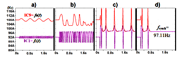Figure 4: Simulation results for KM a1, The instantaneous frequencies f₁(t) and  f₉(t) for the values of the common coupling factor ρ: a) ρ = 1.3Hz; b) ρ = 5Hz; c) ρ = 10.8Hz; d) ρ = ρ_synch = 10.8Hz.

Matlab description for KM a5 differ from KM a1 by replacing coupling coup{1,9}={[ρ 0 1]}; by 2 couplings:

coup{1,5}={[ρ 0 1]};  coup{5,9}={[ρ 0 1]};

Experimental waveforms of the instantaneous frequencies f₁(t), f₅(t) and  f₉(t) are shown in Figure 5, for the similar coupling factors: ρ = 1.05Hz, ρ = 4.2Hz, ρ = 8.35Hz, ρ_synch = 8.41Hz.

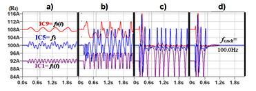Figure 5: Simulation results for KM a5, The instantaneous frequencies f₁(t) and  f₉(t) for the values of the coupling factor ρ: a) ρ = 1.05Hz; b) ρ = 4.2Hz; c) ρ = 8.4Hz; d) ρ = 8.41Hz.

Simulations like Figure 4, 5 were performed for all oscillator ensembles a1-a8 (Fig 3). The obtained numerical characteristics are presented in Table 2. Each column of the table contains:

• the name of the ensemble (N),
• the common coupling factor providing synchronizing (f_ij),
• the deviation of the synchronization frequency from the basic frequency (Δf_syn).

Table 2 Numerical characteristics of oscillator ensembles a1-a8

N	a1	a2	a3	a4	a5	a6	a7	a8
fij	10.86	16.49	8.01	14.36	8.411	13.97	9.15	12.41
fs	97.11	99.79	100.0	99.23	100.0	100.0	100.3	97.08

The second example is a ring sequence (Figure 6a) of 5 oscillators with couplings, which are sequentially switched on with a delay of 5 seconds. The natural frequencies of the oscillators are evenly distributed in the interval [98 – 102] Hz (base frequency – 100 Hz). Each coupling function in an open loop 1–2–3–4–5 contains only the first harmonic with zero phase shift  and coupling factors are =3Hz ( =0.03).

The aim of the numerical experiments is to analyze the dependence of the synchronization process on the magnitude of the coupling function between the first and fifth oscillators ( ).

The initial description of the ring ensemble is presented in Figure 6b for 5-1 coupling factor 0.005. Waveforms of instantaneous frequencies of oscillators obtained as simulation results are presented in Figure 7.

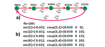Figure 6: a) The ring of 5 coupled harmonic oscillators, b)  matlab description of the ring.

At t < 5sec the instantaneous frequencies of all oscillators coincide with their natural frequencies because all couplings are disabled. After coupling 1-2 is switched on at t = 5sec the second oscillator is synchronized by the natural frequency of the first one. Similarly the synchronization of oscillators 3 , 4 occurs at t = 10sec and at t = 15sec correspondingly. But enabling coupling 4-5 at t = 20sec does not lead to the synchronization of oscillator 5 because the discrepancy of frequencies (f₅ – f₁ = 4Hz) exceeds the coupling factor 3Hz. As a result, the oscillator 5 instantaneous frequency at 20 < t < 25sec is a periodic waveform. Enabling coupling 5-1 closes the ring and interrupts all synchronizations at t > 25 sec where instantaneous frequencies of all oscillators are time varying waveforms.

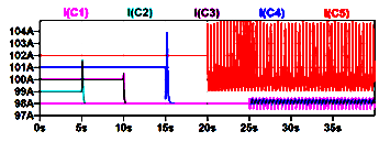Figure 7: Simulation results obtained using matlab description in Figure 6b.

In more details the waveforms at t = 24-28 sec. can be seen in Figure 8a which is the first one of the plots in Figure 8a-e representing simulation results for some values of 5-1 coupling factor . The unsynchronized behavior of the oscillators is seen in two intervals: ≤ 0.041 (Figure 6a,b) and ≥ 0.078  (Figure 6e). In the interval 0.0042 ≤  ≤ 0.077 (Figure 6c-d) all oscillators are mutually synchronized.

Thus, two bifurcation points can be defined in the axis of values of the coupling factor. At  0.00415 the transition from unsynchronized (Figure 8b) to synchronized (Figure 8c) mode occurs. The inverse transition (from Figure 8d to Figure 8e) occurs at  0.0775.

A similar analysis of the impact of the coupling factor was performed for the 5-1coupling function with a non-zero phase shift ( ). The results are shown  in Figure 9.

The input description of the 5-1 coupling is presented as

coup{1,5}={[0.025 0.25 25]};

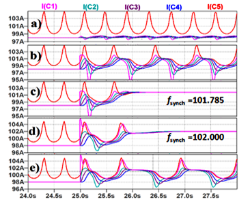Figure 8: Simulation results for various 5-1 coupling factors a) =0.005, b) =0.041, c) =0.042, d) =0.077 e) =0.078.

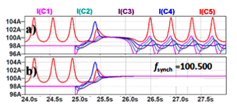Figure 9: Simulation results for various 5-1 coupling factors under phase shift :  a) =0.024, b) =0.025.

Some obtained waveforms in Figure 9 demonstrate the transition from unsynchronized (Figure 9a) to synchronized (Figure 9b) mode in the single bifurcation point ≈0.0245.

The simulated waveforms in Figure 10 are obtained under varying the second harmonic magnitude (  of 5-1 coupling function. The phase shift and all other harmonics of the coupling function are zeroes.

coup{1,5}={[ ] [0.014  0  25]};

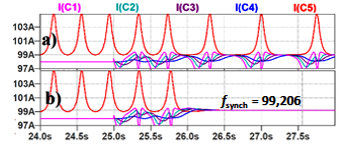Figure 10: Simulation results for 5-1 for coupling function with the second harmonic only ( =0.0): a) =0.014, b) =0.015.

Here similarly to Figure 9 the domains of unsynchronized and synchronized modes are separated by the sole bifurcation point of the second harmonic  .

Thus, the presented experiments showed the useful application of the proposed approach to simulating coupled oscillators.

6. Conclusions

The paper presents the numerical approach to simulate ensembles of arbitrary oscillators. The principles of operation of the required software based on the circuit simulator and the Matlab system are developed.

The proposed approach for analyzing an ensemble of oscillators is based on the construction of model of electrical circuit. The Kirchhoff equations of this model coincide with the Kuramoto model equations of the considered ensemble. The unambiguous correspondence between the currents and voltages of the equivalent circuit and the phases and frequencies of the Kuramoto model is provided. As a result, simulating the equivalent electrical circuit performs the computation of the transients in the ensemble including computation of oscillatory phases and frequencies. The analysis of obtained transients is supported by plotting tools of modern electrical simulators.

The set of simple rules provides constructing of the equivalent circuit for coupling functions defined by their Fourier series. The numerical procedure has been developed to automatically create the input netlist. The routine generates netlist by processing the compact form of user-friendly ensemble description. The description includes lists of oscillator parameters and communication parameters represented as a Matlab structure.

The presented numerical examples have demonstrated the efficiency and convenience of the proposed approach.

Acknowledgment

The reported study was funded by RFBR, project number 19-29-03012

1. M.M. Gourary, S.G. Rusakov, “A Simulation Tool for Analysis of Oscillator Ensembles Defined by Kuramoto Model,” 2020 European Conference on Circuit Theory and Design (ECCTD), Sofia, Bulgaria, 1-4, 2020, doi: 10.1109/ECCTD49232.2020.9218382.
2. S.H. Strogatz, Nonlinear Dynamics and Chaos with Applications to Physics, Biology, Chemistry, and Engineering, Westview Press, 2015. 2, 528. ISBN 978-0-813-34910-7.
3. M. Bonnin, F. Corinto, M. Gilli, “Periodic Oscillations in Weakly Connected Cellular Nonlinear Networks,” IEEE Transactions on Circuits and Systems I: Regular Papers, 55(6), 1671-1684, 2008, doi: 10.1109/TCSI.2008.916460.
4. P. Ashwin, S. Coombes, R.J. Nicks, “Mathematical Frameworks for Oscillatory Network Dynamics in Neuroscience,” Journal of Mathematical Neuroscience 6 (2), 1-92, 2016, doi: 10.1186/s13408-015-0033-6.
5. P. Bhansali, J. Roychowdhury, “Injection Locking Analysis and Simulation of Weakly Coupled Oscillator Networks,” in Simulation and Verification of Electronic and Biological Systems, 71-93, Springer Science+Business Media B.V., 2011, doi: 10.1007/978-94-007-0149-6_4.
6. K.S.T. Alain, F.H. Bertrand, “A Secure Communication Scheme using Generalized Modified Projective Synchronization of Coupled Colpitts Oscillators,” IJMSC, 4 (1), 56-70, 2018, doi: 10.5815/ijmsc.2018.01.04
7. P. Maffezzoni, B. Bahr, Z. Zhang, L. Daniel, “Reducing Phase Noise in Multi-Phase Oscillators,” IEEE Transactions on Circuits and Systems I: Regular Papers, 63(3), 379-388, 2016, doi: 10.1109/TCSI.2016.2525078.
8. C. Gong, A. Pikovsky, “Low-Dimensional Dynamics for Higher Order Harmonic Globally Coupled Phase Oscillator Ensemble”, Physical Review E. 100 (6-1), 062210, 2019, doi: 10.1103/PhysRevE.100.062210.
9. F. Dörfler, F. Bullo, “Synchronization in complex networks of phase oscillators: A survey,” Automatica, 50(6), 1539-1564, 2014. doi: 10.1016/j.automatica.2014.04.012.
10. J.A. Acebron, L.L. Bonilla, C.J.P. Pérez Vicente, F. Ritort and R. Spigler, “The Kuramoto model: A simple paradigm for synchronization phenomena,” Reviews of Modern Physics 77(1), 137 – 185, 2005, doi: https://doi.org/10.1103/RevModPhys.77.137
11. A. Gilat, Matlab: An Introduction with Applications, 7th Edition Pod for Student Choice, John Wiley & Sons, Incorporated, 2017.
12. J. Kim, “Kuramoto model Numerical code (MATLAB),” in
    https://appmath.wordpress.com/2017/07/23/kuramoto-model-numerical-code-matlab
13. “Cleve’s Corner: Cleve Moler on Mathematics and Computing” in
    https://blogs.mathworks.com/cleve/2019/08/26/kuramoto-model-of-synchronized-oscillators/
14. “Python implementation of the Kuramoto model on graphs” in https://github.com/fabridamicelli/kuramoto_model
15. O’Keeffe, K.P., Hong, H. Strogatz, S.H. Oscillators that sync and swarm. Nat Commun 8, 1504 (2017). doi: 10.1038/s41467-017-01190-3
16. K. Ochs, D. Michaelis and J. Roggendorf, “Circuit Synthesis and Electrical Interpretation of Synchronization in the Kuramoto Model,” 2019 30th Irish Signals and Systems Conference (ISSC), Maynooth, Ireland, 1-5, 2019, doi: 10.1109/ISSC.2019.8904942.
17. A. Fettweis, “Wave Digital Filters: Theory and Practice,” Proceedings of the IEEE, 74(2), 270–327, 1986, doi: 10.1109/PROC.1986.13458.
18. Y. Kuramoto “Self-entrainment of a population of coupled non-linear oscillators,” In: Araki H. (eds) International Symposium on Mathematical Problems in Theoretical Physics. Lecture Notes in Physics, 39. Springer, Berlin, Heidelberg, 1975, doi: 10.1007/BFb0013365.
19. S.N. Dorogovtsev, J.F.F. Mendes “Evolution of networks,” Advances in Physics, 51(4), 1079-1187, 2002, doi: 10.1080/00018730110112519
20. F. A. Rodrigues, T.K.DM. Peron, P.Ji, “The Kuramoto model in complex networks,” Physics Reports, 610, 1-98 2016. doi: 10.1016/j.physrep.2015.10.008ted, 2017.
21. A. Arenas, A. Díaz-Guilera, J. Kurths, Y. Moreno, C. Zhou, “Synchronization in complex networks,” Physics Reports, 469(3), 93-153, 2008, doi: 10.1016/j.physrep.2008.09.002.
22. Ben-Avraham, D.A. Barrát, M. Barthélemy, A. Vespignani, “Dynamical Processes on Complex Networks,” J. Stat Phys, 135, 773–774, 2009, doi: 10.1007/s10955-009-9761-x
23. A. Bohn, J. García-Ojalvo, “Synchronization of coupled biological oscillators under spatially heterogeneous environmental forcing,” Journal of Theoretical Biology,” 250(1), 37-47, 2008, doi: 10.1016/j.jtbi.2007.09.036.
24. Y. Kuramoto, D. Battogtokh, “Coexistence of Coherence and Incoherence in Nonlocally Coupled Phase Oscillators,” Nonlinear Phenomena in Complex Systems, 5(4), 380–385, 2002.
25. P. Kumar, D. Verma, D.: Parmananda, P. “Partially synchronized states in an ensemble of chemo-mechanical oscillators,” Physics Letters A. 381(29), 2337-2343, 2017. doi: 10.1016/j.physleta.2017.05.032.
26. M.J. Panaggi and D.M. Abrams, “Chimera states: coexistence of coherence and incoherence in networks of coupled oscillators,” Nonlinearity, 28(3), 2015, doi: 10.1088/0951-7715/28/3/R67.
27. F. Yuan, Injection-locking in mixed-mode signal processing, Springer, New York, 2019.
28. LTspice, in https://www.analog.com/en/design-center/design-tools-and-calculators/ltspice-simulator.html

(Click Here)