1. Introduction

This paper is an extension of two works originally presented in the Proceedings of the Asia-Pacific Signal and Information Processing Association Annual Summit and Conference 2020 (APSIPA ASC) [1] and in the International Florida Artificial Intelligence Society Conference Proceedings (FLAIRS-34) [2]. Both papers study the qualitative behaviour of multivariate fractional Brownian motion by analysing the distribution of up and down encodings in terms of ordinal patterns and permutation entropy.

Time series data is part of many real-world applications, e.g., weather records, patient health evolution metrics, (industrial) sensor data, stock prices, website clicks, server metrics, network data, political or sociological indicators, video or voice messages – just to name a few. Time series can be understood as a series of (realvalued) random variables of a time-dependent system that changes over time, also called a dynamical system. For many real-world applications, modelling time-dependent dynamical systems require specific properties such as long-range dependence or self-similarity. For example, the long memory is fundamental in internet traffic [3] or for financial data [4]. If financial return series exhibit a longrange dependence, this indicates that observed returns over time are not independent. When returns are not independent, past returns may help predict future returns [5]. This work focuses on a special class of dynamical systems or stochastic processes that describe long-range dependence and self-similarity properties, called fractional Brownian motion (fBm) and denoted as B_H(t), where the so-called Hurst parameter H describes the self-similarity.

While classical time series analysis examines the values of the time series themselves, symbolic time series analysis considers a non-parametric mapping or encoding into a sequence of symbols. This is particularly promising in the case of dynamical systems such as fBm, as the overall dynamics of the generating system is uncovered [6]. To measure the qualitative behaviour of a generating system, efficient measures of the sequence of symbols to a set of scalar-valued representations, also called features, that capture specific properties are considered. Entropy, a measure that has its origins in information theory, is promising through an encoding that preserves the information content of an object [7]. PE is a robust, scalar-valued measure for determining the degree of complexity of dynamical systems or observed time series by analysing the distribution of symbolic sequences of ordinal patterns [8]. While the associated entropy is low for a deterministic time series, it approaches its maximum value in case of uncorrelated randomness or high complexity. To distinguish between randomness and complexity, an additional measure is necessary. As a complement to permutation entropy (PE), multi-scale permutation entropy (MSPE) captures the complexity of time series on different time scales [9]. On higher time scales, random noise tends to cancel out, resulting in a low entropy value, where complex signals retain a high entropy value. In this manner, it is possible to gain a deeper insight into the randomness and complexity of a system. Another limitation of PE is the inability to distinguish between different patterns of a given motif in amplitudes. In [10], the author introduce weighted permutation entropy (WPE), which takes into account patterns that differ in amplitudes by assigning weights to each extracted pattern.

The behaviour of PE on fBm in the univariate case is well understood [8, 11, 12]. Not only the PE but also the distributions of ordinal patterns of certain lengths yield interesting properties. The distributions of ordinal patterns of lengths (also called order) two and three yield parameter functions that can be used for descriptive purposes such as autocorrelation. The distribution of order four has irrational values and depends on the noise distribution. The resulting closed formulas for computation are used in this work. The distributions of ordinal patterns of lengths greater than four do not yield closed formulas. Thus, a relationship between autocorrelation or spectrum on the one hand and ordinal patterns, on the other hand, does no longer exist [8]. In [13], the author investigate the behaviour of MSPE on fBm, denoted as B_H(t), and show that MSPE of the fractional Gaussian noise, the increment process of fBm, i.e., X(t) = B_H(t + 1) − B_H(t), is time-scale invariant. In [2] we investigate the behaviour of WPE on fBm and show that the distribution of ordinal patterns of order d = 2 and thus also WPE are independent of the weighting.

Moreover, in many fields of applications, multivariate measurements are performed. Examples of multivariate fractional Brownian motion (mfBm) can be found in economic time series [14], or functional Magnetic Resonance Imaging of several brain regions [15]. This work summarises the behaviour of several multivariate extensions of PE on mfBm. The first original conference paper [1] studies the behaviour of two canonical multivariate extensions of PE, known as pooled permutation entropy (PPE) and multivariate multiscale permutation entropy (MMSPE) of orders d = 2 and d = 3, on mfBm. The second original conference paper [2] investigates the behaviour of multivariate weighted permutation entropy (MWPE) of orders d = 2 and d = 3 on mfBm. We extend original works [1] and [2] by

• a comprehensive review of all existing extensions to multivariate permutation entropy including code for computing on Github^[1] and Python Package Index (PyPI)²,
• a complement in existing theoretical and experimental investigations of PPE, MMSPE and MWPE on mfBm in a variation of its Hurst parameter H, i.e., we fill the gaps by investigating the behaviour of additional orders d = 4 and d = 5 as well as other parameters such as in particular different time delays, time scales and number of variables of mfBms,
• a new study on the behaviour of multivariate ordinal pattern permutation entropy (MOPPE) on mfBm, and
• a comparison of all considered multivariate extensions.

This paper is structured as follows and as visualised in Figure 1. After presenting background on (m)fBm and univariate PE in Section 2, needed for the paper to be self-consistent, we provide in Section 3 a review of multivariate extensions of PE and categorise them according to their approach. Since this paper focuses on canonical extensions, we present all those extensions in detail and provide algorithms for their computations. In Section 4, Section 5, and Section 6 we investigate the behaviour of PPE, MMSPE and MWPE, respectively, on mfBm in variation of the Hurst parameter

H, and we complement the original work with previously mentioned investigations. In Section 7 we present a new study on the behaviour of MOPPE on mfBm in variation to the Hurst parameter H. In Section 8 we compare our findings and show that PPE and MMSPE behave identically for all investigated orders, delays, scales, and the number of variables. In addition, MWPE and MOPPE of orders d > 2 uncover different aspects of mfBm, i.e., amplitudes and crosscorrelations, respectively. In Section 9 we conclude our work with mentioning future work.

2. Background

We shortly formalise fBm and subsequently key concepts of ordinal patterns and PE. We then summarise known results from the application of PE on fBm in the univariate case.

2.1        Multivariate Fractional Brownian Motion

A stochastic process, or more generally a mathematical object that is similar to itself at all scales, is called a fractal. When you zoom in on a fractal, it resembles or looks exactly like the original shape. The mathematical property is called self-similarity and is expressed by the so-called Hurst parameter H ∈ (0,1) in honour of Harold Edwin Hurst [16]. The work described here focuses on a class of special stochastic processes, namely fractional Brownian motion (fBm), involving the properties of self-similarity and long-range dependency.

Definition 2.1 (Fractional Brownian Motion) A stochastic process is called fractional Brownian motion (fBm) with Hurst parameter H ∈ (0,1) and denoted as B_H(t) if it is

1. Gaussian,
2. self-similar, i.e., there exists H ∈ (0,1) such that for any a > 0 it is

where ∼ denotes the equality of probability distributions, and it has

3. stationary increments, i.e., B_H(t) − B_H(s) ∼ B_H(t − s).

In case H = 1/2, fBm corresponds to the ordinary Brownian motion. In case H > 1/2, the process has a persistence property and positively correlated increments, i.e., an upward jump is more likely followed by another upward jump and vice versa, and the process exhibits long-range dependence. For H → 1, the process becomes smoother, less irregular and more trendy. In case H < 1/2, the process has negatively correlated increments and an anti-persistence property. Figure 2 shows three different realisations of fBms of length T = 5000 with different Hurst parameters H ∈ {0.25,0.5,0.75} illustrating the properties mentioned above.

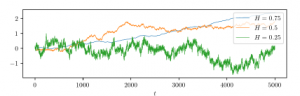
Figure 2: Three different realisations of fBm of length T = 5000 with different H.

Stationarity refers to the fact that the distribution of the process doesn’t change in time, which has important consequences. In particular, the B_H(t) are identically distributed, i.e., the expectation values and variances of components do not depend on time t. Furthermore, the distribution B_H(t) − B_H(s) depends only on t − s, so the correlations of the components also depend only on t − s.

Multivariate generalisations of fBms are introduced in [17, 18] and require an extension of self-similarity to multivariate processes first. While the definition given in [19] concerns a far-reaching generalisation of fBm, where self-similarity becomes operator selfsimilarity for the multivariate case, in [18] the authors restrict themselves to joint self-similarity, where joint self-similarity can be seen as a special case of operator self-similarity where the operator is diagonal. For the sake of simplicity, we focus on the definition introduced in [18].

Definition 2.2 (Multivariate Self-Similar Process) A multivariate process ((Xⁱ,…, X^m(t))_t∈R with variable-

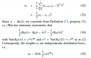
dimension m ∈ N is called self-similar, if there exists a vector H = (H₁,…, H_m) with H_i ∈ (0,1) for i = 1,…,m such that for any a > 0 it holds that

(X¹(at),…, X^m(at))_t∈R ∼ (a^H1 X¹(t),…,a^Hm X^m(t))_t∈R, where ∼ denotes the equality of finite-dimensional distributions.

With Definition 2.2, mfBm is defined as follows.

Definition 2.3 (Multivariate Fractional Brownian Motion [20]) An m-multivariate process (( _R is called multivariate fractional Brownian motion (mfBm) with self-similarity or Hurst parameter H = (H₁,…, H_m) with H_i ∈ (0,1) for i = 1,…,m, and is denoted as B^m_H(t) , if it is

1. Gaussian distributed,
2. self-similar with Hurst parameter H, and it has
3. stationary increments, i.e., B^m_H(t) − B^m_H(s) ∼ B^m_H(t − s).

Multivariate self-similarity imposes some constraints on the covariance structure of mfBm [18]. The covariance structure is characterised by three parameters σ_i > 0, ρ_ij ∈ (−1,1) and η_ij ∈ R for i, j = 1,…,m, which allow two components to be more or less correlated and the process to be reversible in time or not. Parameter σ_i > 0 is the standard deviation of the i-th variable at time t = 1. Parameter ρ_ij = ρ_ji is the correlation coefficient between the variables i and j at time t = 1. Parameters η_ij = −η_ji are antisymmetric and linked with the time-reversibility of mfBm. Multivariate fractional Brownian motion can be characterised by its covariances and cross-covariances of its variables as follows.

Lemma 2.1 (Covariance Function of mfBm [21]) The mfBm B^m_H(t) is marginally an fBm, such that the covariance function

of the i-th variable Bⁱ_Hi of mBfm is as in the univariate case, i.e.,

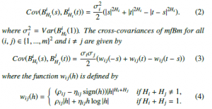
Moreover, the setting of ρ_ij = 1 and η_ij = 0 in (3) and (4) matches with the definition in the univariate case in (2). For m = 1, Definition 2.3 matches with the univariate Definition 2.1 of fBm. Figure 3 shows three realisations of mfBm of length T = 2000, ρ_i,j = 0.3, η_i,j = 0.1/(1 − H_i − H_j) with different Hurst parameters.

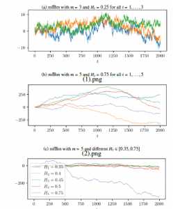
Figure 3: Three different realisations of mfBm with different Hurst parameters.

2.2        Ordinal Pattern Representations

To investigate the qualitative behaviour of mfBm, we use ordinal pattern symbols. Before we get into the details of multivariate ordinal patterns, we introduce univariate concepts.

2.2.1    Ordinal Pattern Symbolisation

In the mathematical theory of symbolic dynamics, a dynamical system is modelled by a discrete space consisting of infinite (sequences of) abstract symbols. These sequences of symbols are the subject of advanced analysis such as entropies. As far as current research is concerned, there are two general approaches to encode the sequence of real-valued measurements into a sequence of symbols as visualised in Figure 4.

On the one hand, classical symbolisation approaches partition the data range according to specified mapping rules in order to then encode a numerical time series into a sequence of discrete symbols from a predefined alphabet Σ. An example of the partitioning of a data range can be found in Figure 4a, while the assignment of the symbols (encoding) to the time series is visualised in Figure 4b. A corresponding and well-known algorithm for determining data range partitions is Symbolic Aggregate ApproXimation (SAX) presented in [22]. On the other hand, ordinal pattern symbolisation is another approach that, independent of the data range of the time series, encodes the total order between two or more neighbours (x < y or x > y) into symbols. This ordinal pattern approach is based on the idea of Bandt and Pompe [23] and visualised in Figures 4c and 4d. Since we use the ordinal symbolisation scheme in the remainder of this work, we present its formalism and advantages in detail in the following.

Ordinal patterns describe the total order between two or more neighbours encoded by permutations.

Definition 2.4 (Univariate Ordinal Pattern)

A vector (x₁,…, x_d) ∈ R^d has ordinal pattern (r₁,…,r_d) ∈ N^d of order d ∈ N if x_r1 ≥ · · · ≥ x_rd and r_l−1 > r_l in the case x_rl−1 = x_rl .

Note that equality of two values within a pattern is not allowed. In this case, without loss of generality, the newer value is replaced with a smaller value. Figure 4c shows all possible ordinal patterns of order d = 3 of a vector (x₁, x₂, x₃). To symbolise a time series (x₁, x₂,…, x_T) ∈ R^T each point in time t ∈ {d,…,T} is assigned its ordinal pattern of order d. The order d is chosen to be much smaller than the total length T of the time series to look at smaller ordinal pattern windows within the series and their distributions of “up and down” movements. To assess the overarching trend, delayed behaviour is of interest. The time delay τ ∈ N is the delay between successive points in the symbol sequences. Different delays show different details of the structure of a time series. Figure 4d visualises ordinal pattern determination of order d = 3 and time delay τ = 1 of three different time points in a time series marked in blue, orange and magenta. Note that ordinal patterns are determined at any arbitrary point in time.

The ordinal approach has notable advantages in its practical application. First of all, the method is conceptually simple as it reflects man’s natural thought of up and down movements and is, therefore, open to interpretation. Second, prior knowledge of the data range or the type of time series is not necessary. The concept can be applied to any time series as long as the range of values is ordered, e.g. x_t ∈ R. Third, the ordinal approach supports robust and fast implementations [24, 25]. Fourth, it allows for an easier estimation of a good symbolisation scheme compared to the classical symbolisation approaches [26, 27].

2.2.2    Permutation Entropy

Not the ordinal patterns themselves, but their distributions in a univariate time series (x_t)^T_t=1 are of interest. Thus, each pattern is identified with exactly one of the ordinal pattern symbols j = 1,2,…,d!. To assess the (dis)order of the identified symbols in the system or in the time series, we use a measure of the dispersion from the field of statistics, namely entropy. The greater the disorder, the higher the entropy. The statistical interpretation of entropy corresponds to Shannon’s information entropy used in information theory or computer science. Applying the well-known formula for (Shannon) entropy

where Z is an alphabet of symbols Z = {z₁,z₂,…,z_n} to ordinal pattern symbols leads directly to the definition of permutation entropy.

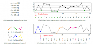
Figure 4: Two approaches for symbolising a univariate time series: (a) and (b) classical symbolisation and (c) and (d) ordinal pattern symbolisation. Best viewed in colour.

Definition 2.5 (Permutation Entropy [23])

Permutation entropy (PE) of order d ∈ N and delay τ ∈ N of a univariate time series x N is defined by

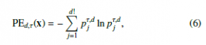
where p^τ,_j ^d is the frequency of occurrence of ordinal pattern j in the time series.

In time series with maximally random ordinal pattern symbols, the ordinal patterns are equally distributed so that PE is ln(d!). For a time series with a regular pattern, e.g., in the case of strict monotony, PE is equal to zero [7].

2.2.3     Multi-Scale-Permutation Entropy

For example, biological and physiological time series, as well as time series from other fields, often contain complex correlations between both temporal and spatial levels (scales) that need to be uncovered. PE achieves a maximum entropy value both on completely random time series and on series with complex correlations based on a determinism. To uncover multi-scale complex correlations, multi-scale entropy (MSE) proposed in [28] provides a systematic procedure to assign small complexity values to both fully predictable and fully random uncorrelated time series. In contrast, correlated processes across different scales have a high complexity value. In [9], the author extend the concept of MSE to univariate ordinal patterns.

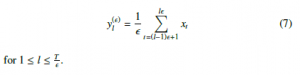
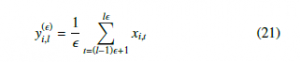
For the consideration of different scales of a time series and an associated definition of MSPE, a coarse-grained procedure is used:

From the original time series, several consecutive time data points are averaged within a non-overlapping time window of scaling length , also called scaling factor. Each element of the coarsegrained time series y = (y⁽_l⁾)^T_l=^/₁ is calculated as:

Definition 2.6 (Multi-Scale Permutation Entropy [9])

Multi-scale permutation entropy (MSPE) of order d ∈ N and delay τ ∈ N of a univariate time series x N is defined as PE of its coarse-grained time series y = (y_l )_l=^/₁ , that is

2.2.4    Weighted Permutation Entropy

Another shortcoming in the above Definition 2.5 of PE is that when the ordinal patterns are extracted, no information other than the order structure is preserved. In particular, information about the amplitude in a time series is lost. However, ordinal patterns with large differences in amplitude should contribute in different ways to the computation of PE. The weighted permutation entropy introduced in [10] allows for the weighting of ordinal patterns by exploiting amplitude information resulting from small fluctuations in the time series due to the effect of noise to be weighted less than ordinal patterns with large amplitudes.

Definition 2.7 (Weighted Permutation Entropy [10])

Weighted permutation entropy (WPE) of order d ∈ N and delay τ ∈ N of a univariate time series x N is defined as

2.3        On the Behaviour of Permutation Entropy on Fractional Brownian Motion

This work investigates the behaviour of PE on fBm in a multivariate setting. To this purpose, we recapitulate univariate results from [8]. They investigate the distribution of ordinal patterns in fBm of different orders and, if possible, provide closed formulas for computation of pattern distributions as follows:

Order d = 2.       The ordinal patterns are equally distributed, more

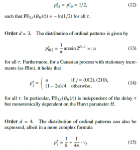
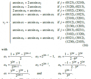
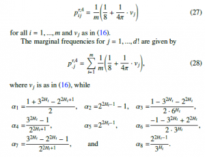
In particular, PE_4,τ(B_H(t)) is independent of the delay τ but monotonically dependent on the Hurst parameter H.

Order d ≥ 5.       There are no closed formulas.

The formulas for the distribution of univariate order patterns of different orders lead to the following behaviour of PE and its extensions MSPE and WPE on fBm. Theorem 2.2 For order d = 2, it holds

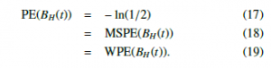
for all delays τ ∈ N and all scales .

Proof. Equation (17) follows directly from (12). Equations (18) or

(19) are shown in [1] and [2], respectively. The independence of

MSPE from the scale  follows from the invariance of the coarsegrained procedure of fBm.

Theorem 2.3 For orders d = 3 and d = 4, PE(B_H(t)) and

MSPE(B_H(t)) are independent of all delays τ ∈ N but monotonically dependent on the Hurst parameter H. Moreover, MSPE(B_H(t)) is independent of all scales , and thus PE(B_H(t)) and MSPE(B_H(t)) are identical.

Proof. The independence of MSPE from the scale  follows from the invariance of the coarse grain procedure of fBm and is shown in [1]. Thus, independence of the delay τ and the dependence on the Hurst parameter H follows directly from (13).

In [2] we observe that for WPE of order d = 3, certain ordinal patterns, namely the strictly ascending ordinal pattern (012) and the strictly descending pattern (210), have higher weights and thus have more impact on the computation of WPE than the other four ordinal patterns. As a result, WPE decreases faster than PE for increasing Hurst parameter H. We elaborate on this experimental discovery in Section 6.

3. A Review of Multivariate Permutation Entropy

This section provides a comprehensive overview of existing extensions of permutation entropy to the multivariate case. We categorise existing multivariate extensions according to their procedure before presenting them in detail.

3.1        Different Approaches for Multivariate Permutation Entropy

A multivariate time series ((x_tⁱ)^m_i=1)^T_t=1 such as a certain realisation of mfBm has more than one time dependent variable. Each variable xⁱ for i ∈ 1,…,m not only depends on the respective past values in time but also has some dependence on other variables in phase space.

Considering two time points (x_tⁱ)^m_i=1 and (x_tⁱ₊₁)^m_i=1 with m variables, simply put two vectors, it is not possible to establish a total order between them. A total order is only possible if ^x_tⁱ > ^x_tⁱ₊₁ or ^x_tⁱ < ^x_tⁱ₊₁ for all i ∈ 1,…,m. Therefore, there is no trivial generalisation of the PE algorithm to the multivariate case.

Nevertheless, numerous studies deal with the multivariate extensions of PE. We classify proposed extensions into four procedures.

The multivariate time series is

1. projected into univariate ordinal space by determining univariate ordinal pattern between neighbouring values in time space (row marked in red in Figure 5a) in each single variable i , and then pooled over all m variables for multidimensionality, or
2. projected into univariate ordinal space by determining univariate ordinal pattern between values of all m variables (column marked in red in Figure 5b) for each single time point t, and then pooled over all T time points for multidimensionality, or c) projected into multivariate ordinal space by determining the multivariate ordinal pattern between d vectors of variable dimension m (box marked in blue in Figure 5c for d = 2), or
3. d) projected onto a single-dimensional reduction first (box marked in green in Figure 5d), and then transformed into ordinal space by determining univariate ordinal pattern.

The first procedure a) is a canonical extension of the univariate definition and is presented in [29] as pooled permutation entropy (PPE). PPE is probably the most widely used multivariate extension. While PPE measures the complexity of each variable in time space, procedure b) analyses the complexity of the variables in phase space. A variant of procedure b) is introduced in [30] as Multivariate Permutation Entropy (MvPE). The third procedure c) first requires an extension of univariate ordinal pattern to multidimensionality. Some theoretical basis for this is set in [31, 32]. A detailed discussion and challenge on real-world data can be found in [33]. The idea of the fourth procedure d) is to first reduce the number of variables m to a single dimension, i.e., m = 1, by applying a distance measure or dimension reduction algorithm. Consequently, Definition 2.5 can then be used for PE computation directly. Rayan, i n[34], the author propose several distance measures to reduce the dimensionality, that is Euclidian distance with reference point (^x_tⁱ₌₀)^m_i=1, Manhattan distance with reference point (^x_tⁱ₌₀)^m_i=1, and Euclidian distance with reference point 0. To consider correlations between variables in space, in [33], the author propose to reduce the dimension using principal component analysis.

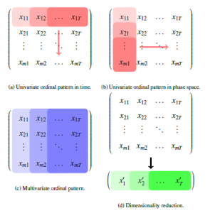
Figure 5: Four procedures of ordinal pattern determination in a multivariate time series.

Since the determination of ordinal patterns in both procedures b) and d) requires transformations of the structure of mfBms, we restrict ourselves in the following to extensions a) and c) that are some kind of canonical extensions.

3.2        Pooled Permutation Entropy and Adaptions

The procedure in Figure 5a is a canonical extension of PE to the multivariate case, i.e., univariate ordinal patterns are determined for each variable of the multivariate time series before each pattern of all variables is pooled. This idea is introduced in [29] and referred to as pooled permutation entropy (PPE). In addition, we introduce two adaptations based on PPE that take into account different aspects of a time series, i.e., different scales or amplitudes, called multivariate multi-scale permutation entropy (MMSPE) or multivariate weighted permutation entropy (MWPE), respectively.

3.2.1    Pooled Permutation Entropy

The idea of PPE is to use marginal frequencies of d! ordinal patterns regarding all m variables as input for entropy computation. For the determination of marginal frequencies, an auxiliary matrix has to be established first as follows.

1. For each variable i = 1,..,m and for each ordinal pattern j = 1,…,d!, count all time steps s ∈ [τ(d − 1) + 1,T], for which the variable-time pair (i, s) has the ordinal pattern j.
2. Divide the counts by m δ, where δ := T − τ(d − 1) is the total count of ordinal patterns each variable has.
3. Store the results, i.e., frequencies p^τ,_ij^d in a so-called pooling matrix P ∈ (0,1)^m×d!, which reflects the distribution of ordinal patterns in the multivariate time series across its m

It holds ^Pm_i=1 ^Pd_j=^! ₁ p^τ,_ij^d = 1. For computational reasons, marginal frequencies p^τ,_.j^d = ^Pm_i=1 p^τ,_ij^d must not vanish for j = 1,…,d!. If they vanish, set the value close to zero.

Definition 3.1 (Pooled Permutation Entropy [29]) Pooled permutation entropy (PPE) of a multivariate time series

X = ((x_tⁱ)^m_i=1)^T_t=1 is defined as PE of the marginal frequencies

p^τ,_.j^d = ^Pm_i=1 p^τ,_ij^d for j = 1,…,d! describing the distribution of the ordinal pattern and can be calculated as

In the literature, PPE is often referred to as Multivariate Permutation Entropy. To avoid confusion with other multivariate versions, we use the original naming. A major advantage of PPE is that within the procedure also univariate PE can be derived for each variable by calculating the PE based on the frequencies p_ij of all ordinal patterns j = 1,…,d! for corresponding i = 1,…,m, i.e. row by row on the pooling matrix. Algorithm 1 provides pseudocode for computing PPE.

Algorithm 1: Computation of PPE

Input: Multivariate Time Series X^m×T, Order d, Delay τ Function pooling(X,d,τ):

P^m×d! ← pooling matrix initialised with zeros for every time series variable i = 1,…,m in X do for each ordinal pattern j = 1,…,d! do

c ← number of time steps s ∈ [τ(d − 1) + 1,T] with pattern j

P_ij ← divide c by the number of total time steps δ · m in the multivariate time series X return P

Function marginalisation(P): p^1×d! ← vector of marginalisation initialised with zeros

for every column j = 1,…,d! in P^m×d! do

p_j ← sum up p_ij

return p

return PE(p)

For example, PPE is successfully used in the analysis of electroencephalography (EEG) signals, as cross-channel regularities between spatially distant variables, i.e., on different hemispheres or in different areas, can be extracted by long-range spatial nonlinear correlations [29]. Furthermore, in [24], the author successfully used PPE to study the 19-channel scalp EEG reflecting changes in brain dynamics of a boy with lesions predominantly in the left temporal lobe caused by connatal toxoplasmosis. In [35], the author use PPE to characterise sleep EEG signals from more than 80 hours of nocturnal sleep recordings and classify sleep stages. They find that each sleep stage is characterised by statistically different PPE values and that the observed pattern of PPE is consistent with the physiological properties of the EEG in each sleep stage.

3.2.2    Multivariate Multi-Scale Permutation Entropy

In addition to PPE and by analogy with MSPE, Morabito et al. [9] provide a canonical definition of multivariate multi-scale permutation entropy. MSPE and MMSPE are calculated on different time scales by processing the coarse-grained time series as a function of the scale factor . Per variable i in a multivariate time series, several consecutive time data points are averaged within a nonoverlapping time window of the scaling length . Each element of

the coarse-grained time series Y = ((^y(_i,l^))T_l=^/₁ )^m_i=1 is calculated as:

for all i = 1,…,m and 1.

Definition 3.2 (Multivariate Multi-Scale PE [9]) Multivariate multi-scale permutation entropy (MMSPE) of order d ∈ N and delay τ ∈ N of a multivariate time series X is defined as PPE of its coarse-grained time series Y, that is

The simultaneous utilisation of a multi-scale approach and the consideration of multiple variables of the time series facilitates assessing the complexity of the underlying dynamical system. Algorithm 2 provides pseudocode for computing MMSPE.

Algorithm 2: Computation of MMSPE

Input: Multivariate Time Series X^m×T, Order d, Delay τ,

Scale Factor

Y^m×(T/) ← coarse-grained multivariate time series initialized with zeros

for every time series variable i = 1,…,m in X do y ← calculate coarse-grained univariate time series

3.2.3    Multivariate Weighted Permutation Entropy

In addition to PPE and by analogy with WPE, in [2] we provide a canonical definition of multivariate weighted permutation entropy. Again, for the determination of MWPE, an auxiliary matrix has to be established first:

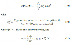
1. For each variable i = 1,..,m and for each ordinal pattern j = 1,…,d!, select all time steps s ∈ [τ(d − 1) + 1,T] for which the variable-time pair (i, s) has the ordinal pattern j.
2. Add up the weights w_t, i.e., w_ij = ^PT_t=dτ₋τ₊₁ w_t for all selected ordinal pattern vectors j and for each variable i = 1,…,m. Note that the total count of weights wⁱ_t for each variable i is δ := T − (dτ − τ).
3. Divide the weighted sum w_ij by the total sum of all m δ weights to obtain the weighted frequencies for every ordinal pattern j.
4. Store the results, i.e., weighted frequencies p^τ,_wij^d in a so-called weighted pooling matrix P^τ,_w^d ∈ R^m×d!, which reflects the weighted distribution of ordinal patterns in the multivariate time series across its m

Based on the weighted pooling matrix P^τ,_w^d, multivariate weighted permutation entropy can be calculated as follows.

Definition 3.3 (Multivariate Weighted PE [2]) Multivariate weighted permutation entropy (MWPE) of a multivariate time series X = ((x_tⁱ)^m_i=1)^T_t=1 is defined as PE of the marginal weighted frequencies p_w^τ,_·^d_j = ^Pm_i=1 p^τ,_wij^d for j = 1,…,d! describing the distribution of the weighted ordinal pattern and can be calculated as

Algorithm 3 provides pseudocode for computing MWPE.

Algorithm 3: Computation of MWPE

Input: Multivariate Time Series X^m×T, Order d, Delay τ Function weightedPooling(X,d,τ):

P^m×d! ← weighted pooling matrix initialised with zeros for every time series variable i = 1,…,m in X do

for each ordinal pattern j = 1,…,d! do

w_ij ← add up weights w_t // see Eq.(11) p_ij ← divide w_ij by the total sum of all m · δ

weights return P p ← marginalisation(P)

return PE(p)

3.3        Multivariate Ordinal Pattern Permutation Entropy

A multivariate time series ((x_tⁱ)^m_i=1)^T_t=1 and its corresponding data matrix X ∈ R^m×T has more than one time-dependent variable. Each variable xⁱ for i ∈ 1,…,m not only depends on the respective past values in time but also has some dependence on other variables in phase space. Since all procedures from the previous section consider univariate ordinal patterns per variable i separately, interdependence is not considered. To involve interdependence, an intuitive idea introduced in [33] is to store the univariate ordinal patterns of all variables at a time point t together into one common multivariate ordinal pattern.

Definition 3.4 (Multivariate Ordinal Pattern) A             data        matrix (x₁,…, x_d) ∈ R^m×d has multivariate ordinal pattern

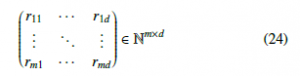
of order d ∈ N if x_ri1 ≥ … ≥ x_rid for all i = 1,…,m and r_il−1 > r_il in

the case xril−1 = xril .

Figure 6 shows all possible multivariate ordinal patterns of order d = 3 and number of variables m = 2.

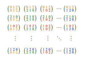
Figure 6: All possible multivariate ordinal patterns of order d = 3 with m = 2 variables. Best viewed in colour.

With the natural extension of univariate ordinal pattern, which leads to Definition 3.4, it is possible to apply the PE algorithm from Definition 2.5 to multivariate time series in its original form.

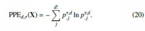
Definition 3.5 (Multivariate Ordinal Pattern PE [33]) Multivariate ordinal pattern permutation entropy (MOPPE) of order d ∈ N and delay τ ∈ N of a multivariate time series X = ((x_tⁱ)_i^m₌₁)^T_t=1 is defined by

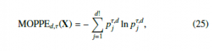
where p^τ,_j ^d is the frequency of multivariate ordinal pattern j in the multivariate time series.

Algorithms 1, 2, 3 and 4 for computing PPE,MMSPE, MWPE and MOPPE, respectively, can also be found on Github¹ and PyPI².

Algorithm 4: Computation of MOPPE

Input: Multivariate Time Series X^m×T, Order d, Delay τ p^1×d! ← frequencies initialised with zeros

for every time step t in X do

for each ordinal pattern j = 1,…,d! do

c ← count all time points t with multivariate ordinal pattern j // see Def. 3.4 p_j ← divide c by the number of total time steps T − τ(d − 1) in the multivariate time series X return PE(p)

The number of the possible multivariate ordinal pattern increases exponentially with the number of variables m, i.e., (d!)^m. Therefore, if d and m are too large, depending on the application, each pattern occurs only rarely or some not at all, resulting in a uniform distribution of ordinal patterns. This has the consequence that subsequent learning procedures may fail. Nevertheless, for small order d and sufficiently large length T of the time series, the use of multivariate ordinal patterns can lead to higher accuracy in learning tasks, e.g., classification [33], because they incorporate interdependence.

4. PPE Applied to mfBm

In this section, we investigate the behaviour of PPE of different orders and delays on mfBm in the variation of its Hurst parameter from both theoretical and experimental points of view. For the sake of completeness, we recapitulate results from previous work and fill in gaps with further results.

4.1        Theoretical Analysis

Orders 2 and 3. In previous work, [1] we show that for order d = 2 the PPE of mfBm is constant for all delays τ as well as any number of variables m, in particular, it holds that

for all τ,m. Furthermore, we show that for order d = 3, the PPE of mfBm stays also independent of the delay τ, but depends monotonically on the number of variables m as well as the Hurst parameter H. In the case H_i = H_j for all variables i, j, PPE is also independent of the number of variables m. Details and corresponding formulas for entropy calculation can be found in the original paper [1].

Orders greater than 3. In this work, we show that a behaviour analogous to that of PPE with order d = 3 can be transferred to orders d > 3.

Theorem 4.1 PPE(B^m_H(t)) of order d = 4 is independent of all delays τ but monotonically dependent on the number of variables m and the Hurst parameter H of mfBm. In the case H_i = H_j for all i, j, it is independent on the number of variables m.

Proof. Let d = 4. Since mfBm B^m_H(t) is marginally an fBm B_H(t), we conclude from Definition 2.3 and (15), that

Considering the distribution of all possible realisations of fBm, we see from the use of (28) in Definition 3.1 that the number of variables m in the case of H_i = H_j for all i, j cancels out. Thus, PPE(B^m_H(t)) is independent of the number of variables m. In addition, PPE(B^m_H(t)) stays independent of all delays τ. Monotonic dependence on the Hurst parameter H is preserved since the transformations carried out, i.e. additions, do not change the monotonicity.

For order d > 4, no closed formulas for the distribution of ordinal patterns in fBm exist (see Section 2.3). Nevertheless, analogous behaviour can also be observed in this case, and we we evaluate that in an experimental setting in the next section.

4.2        Experimental Evaluation

In this experimental evaluation, we investigate the behaviour of PPE on mfBm in the variation of the Hurst parameter H, the number of variables m and the delay τ. All experimental computations are based on simulations of mfBms using an algorithm described in [20] with parameters H_i = H_j for all i, j, ρ_i,j = 0.0 and η_i,j = 0.1/(1 − H_i − H_j) for Lemma 2.1. The lengths T = 10,000 of mfBms are assumed to be large. The results of computations are visualised in Figure 7.

In Figure 7a we show the independence of PPE of all orders d = 2 (green), d = 3 (orange), d = 4 (blue), and d = 5 (red) on mfBm from number of variables m. For this, the delay is fixed to τ = 1. All green lines, i.e., for d = 2, are constant, namely − ln(1/2), for each m, confirming the independence of numbers of variables m in (26). All other lines, i.e., for d > 2, are also the same for any m, but monotonically dependent on the Hurst parameter H, i.e., in particular confirming Theorem 4.1. In Figure 7b we show the independence of PPE on mfBm from delay τ. For this, the number of variables is fixed to m = 3. Again, all green lines, i.e., for d = 2, are constant − ln(1/2) for each τ, confirming the independence of delay τ in (26). All other lines, i.e., for d > 2, are also the same for any τ, but monotonically dependent on the Hurst parameter H, in particular confirming Theorem 4.1.

The deviations of the values of PPE in Figure 7 with increasing Hurst parameter H thus result from the length restriction in the simulation, i.e., the distributions as given in the theoretical part are only to be expected if T → ∞ converges [13]. Thus, for a small length T, the estimates of the probabilities for the ordinal patterns differ from the true values of a hypothetical mfBm of infinite length. All in all, the experiment underpins our theoretical results. The results are not surprising since PPE pools over the univariate patterns so that mfBm can be understood by the computational logic as a kind of extended univariate fBm. This kind of extension ensures that the deviations for greater Hurst parameter H and larger number of variables become smaller and can also be observed in Figure 7a.

5. MMSPE Applied to mfBm

In this section, we investigate the behaviour of MMSPE of different orders, delays, and scales on mfBm in the variation of its Hurst parameter from both theoretical and experimental points of view. For the sake of completeness, we recapitulate results from previous work and fill in remaining results.

5.1        Theoretical Analysis

To investigate the behaviour of MMSPE on mfBm, coarse-grained fractional Brownian motion has to be considered. By using (7)

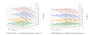
Figure 7: Experimental computations of PPE of orders d = 2 (green), d = 3 (orange), d = 4 (blue), and d = 5 (red) on mfBm in variation of its Hurst parameters H.

or (21) on fBm, coarse-grained fractional Brownian motion (cfBm) is defined as

In [1] we show that the structure of the covariance function is the same as the original fBm for all variables i = 1,…,m, but with additional information of the scale factor . Therefore the covariance function of the original fBm or mfBm is invariant to the coarse-grained procedure. For this reason, the results from the previous Section 4 are directly transferable to MMSPE.

Orders 2 and 3. For order d = 2 the MMSPE on mfBm is constant for all delays τ, number of variables m, as well as any scales . In particular holds

for all τ,m,. Furthermore, for order d = 3, the MMSPE on mfBm is also independent of delays τ and scales  but depends monotonically on the number of variables m as well as the Hurst parameter H of mfBm. In the case H_i = H_j for all variables i, j, MMSPE is also independent of the number of variables m. Details and corresponding formulas for entropy calculation can be found in the original work [1].

Orders greater than 3. With previous insights, the transfer of results from MMSPE of order d = 3 to MMSPE of order d = 4 is straightforward. For the sake of completeness, we formulate the following theorem.

Theorem 5.1 MMSPE(B^m_H(t)) of order d = 4 is independent of all delays τ and scales , but monotonically dependent on the number of variables m and Hurst parameter H of mfBm. In the case H_i = H_j for all i, j, it is independent on the number of variables m.

Proof. For mfBm, each variable i = 1,…,m is marginally an fBm. Since the covariance function of fBm is invariant to the coarsegrained procedure in (29), the independence of scales  follows [1]. Then Theorem 4.1 is directly applicable, which implies independence from the delay τ, the number of variables m and monotonic dependence on the Hurst parameter H.

For order d > 4, no closed formulas for the distribution of ordinal patterns in fBm exist (see Section 2.3). Nevertheless, analogous behaviour can also be observed in this case. We evaluate this behaviour in an experimental setting in the next section.

Summarising the results of this subsection, the inclusion of different scales in mfBm has no influence. This is particularly related to or reflects the fractal property because it resembles the original shape when a fractal is zoomed in or scaled. Thus, MMSPE and PPE show identical behaviour, which we investigate and discuss in detail in Section 8.

5.2        Experimental Evaluation

In this experimental evaluation, we investigate the behaviour of MMSPE on mfBm in the variation of the Hurst parameter H, delay τ, number of variables m, as well as scale . The experimental computations are based on the same simulations of mfBms as in Section 4.2.

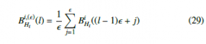
In Figure 8a we show the independence of MMSPE of all orders d = 2 (green), d = 3 (orange), d = 4 (blue), and d = 5 (red) on mfBm from number of variables m. For this, the delay is fixed to τ = 1, and the scale is fixed to  = 2. All green lines, i.e., for d = 2, are constant, namely − ln(1/2), for each m, confirming the independence of numbers of variables m in (30). All other lines, i.e., for d > 2, are also the same for any m, but monotonically dependent on the Hurst parameter H, in particular confirming Theorem 5.1. In Figure 8b we show the independence of MMSPE on mfBm from delay τ. For this, the number of variables is fixed to m = 3, and the scale is fixed to  = 2. Again, all green lines, i.e., for d = 2, are constant with value − ln(1/2) for each τ, confirming the independence of delay τ in (30). All other lines, i.e., for d > 2, are also the same for any τ, but monotonically dependent on the Hurst parameter H, in particular confirming Theorem 5.1.

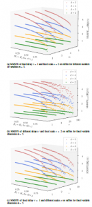
Figure 8: Experimental computations of MMSPE of orders d = 2 (green), d = 3 (orange), d = 4 (blue), and d = 5 (red) on mfBm in variation of its Hurst parameters H.

In Figure 8c we show the independence of MMSPE on mfBm from scale . For this, the number of variables is fixed to m = 3 and the delay to τ = 1. Again, all green lines, i.e., for d = 2, are constant with value − ln(1/2) for each , confirming the independence of scale  in (30). All other lines, i.e., for d > 2, are also the same for any scale , but monotonically dependent on the Hurst parameter H, in particular confirming Theorem 5.1. Again, the reason for the deviations of the values of MMSPE in Figure 8 with increasing Hurst parameter H is the same as in the previous Section 4, namely from length restriction T < ∞ of mfBm.

All in all, the experiment underpins our theoretical results from Since MMSPE is based on PPE and scaling has no influence on mfBm, the behaviour of MMSPE on mfBm in Figure 8 is to be expected the same as that of PPE in Figure 7. A direct comparison is discussed in Section 8.

6. MWPE Applied to mfBm

In this section, we investigate the behaviour of MWPE of different orders and delays on mfBm in the variation of its Hurst parameter from both theoretical and experimental points of view. For the sake of completeness, we recap results from past work and add some further results to fill in some of the remaining research gaps.

6.1        Theoretical Analysis

Order 2. In previous work, [2] we show that for order d = 2, PPE of mfBm is constant for all delays τ as well as numbers of variables m.

Theorem 6.1 MWPE of order d = 2 on mfBm B_H(t) is given by

for all τ,m.

Proof. From [2]: WPE or MWPE differs from PE or PPE, respectively, in that the ordinal patterns are weighted depending on their position t according to (11). For a weight w_t of order d = 2, i.e., of two time steps x_t−τ and x_t, we have

Considering the distribution of all possible realisations of fBm, we see from the use of the weights w_t from (11) in the computation of WPE that the weights cancel out for a constant delay τ ∈ N. With

(12) it follows that WPE(B_H(t)) = − ln(1/2).

Calculating the frequencies of ordinal patterns for the weighted pooling matrix P^τ,_w^d ∈ R^m×d! results in an equal distribution with

for j = {(0,1),(1,0)}. Hence the claim follows.

Orders greater than 2. For orders d = 3 and d = 4, the following theorem can be derived by inspecting corresponding weights of ordinal patterns in combination with results from PPE.

Theorem 6.2 MWPE(B^m_H(t)) of orders d = 3 and d = 4 are independent of all delays τ but monotonically dependent on the number of variables m and Hurst parameter H of mfBm. In the case H_i = H_j for all i, j, it is independent on the number of variables m.

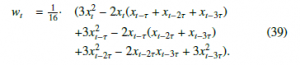
Proof. The weights for ordinal patterns of order d = 3 are given by

In contrast to d = 2, in particular in contrast to (33), due to the lack of symmetry, the weights depend on the time t, and therefore do not cancel and thus influence the value of MWPE. Since the distribution of the ordinal pattern is independent of the weights w_t, the independence of the delay τ is retained. In addition, the multiplication of weights w_t and counts do not affect the monotony that follows from (13) and (14) of PPE. The independence of MWPE from the number of variables m for H_i = H_j for all variables i, j follows with the same line of reasoning as from the end of the proof of Theorem 4.1 when calculating the marginal frequencies.

The weights for ordinal patterns of order d = 4 are given by

Using the same reasoning as in the case of d = 3 and with (15), the independence of the delay τ, the number of variables m and the monotonic dependence of the Hurst parameter H for MWPE are preserved.

For order d > 4, no closed formulas for the distribution of ordinal patterns in fBm exist (see Section 2.3). Nevertheless, analogous behaviour can also be observed in this case, which we evaluate in an experimental setting in the next section.

For increasing Hurst parameter H → 1, m(fBm) is more positively correlated, i.e., after an upward jump, a further upward jump is more likely to follow and vice versa. Consequently, it is more likely that the strictly ascending ordinal pattern (0,1,2) or the strictly descending ordinal pattern (2,1,0) occurs than the other four ordinal patterns (0,2,1), (1,0,2), (2,0,1) and (1,2,0). Since for H → 1 and t → ∞ m(fBm) becomes trendier, the weights of (0,1,2) and (2,1,0) respectively must be larger on average. Thus, by weighting the ordinal patterns of orders d > 2, the values of MWPE are expected to decrease faster than the values of PPE.

6.2        Experimental Evaluation

In this experimental evaluation, we investigate the behaviour of MWPE on mfBm in the variation of Hurst parameter H, delay τ, and the number of variables m. The experimental computations are based on the same simulations of mfBms as in Section 4.2.

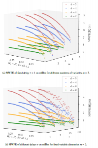
Figure 9: Experimental computations of MWPE of orders d = 2 (green), d = 3 (orange), d = 4 (blue), and d = 5 (red) on mfBm in variation of its Hurst parameters H.

In Figure 9a we show the independence of MWPE of all orders d = 2 (green), d = 3 (orange), d = 4 (blue), and d = 5 (red) on mfBm from number of variables m. For this experiment, the delay is fixed to τ = 1. All green lines, i.e., for d = 2, are constant, namely − ln(1/2), for each m, confirming the independence of numbers of variables m in (31). All other lines, i.e., for d > 2, are the same for any number of variables m, but monotonically dependent on the Hurst parameter H. In Figure 9b we show the independence of MWPE on mfBm from delay τ. For this experiment, the number of variables is fixed to m = 3. Again, all green lines, i.e., for d = 2, are constant with value − ln(1/2) for each delay τ, confirming the independence of delay τ in (31). All other lines, i.e., for d > 2, are also the same for any delay τ, but monotonically dependent on the Hurst parameter H. The reason for the deviations of the values of MWPE in Figure 9 with increasing Hurst parameter H is the same as in the previous Section 4, i.e., the deviations are caused by length constraint T < ∞ of mfBm.

All in all, the experiment underpins our theoretical results statet in Theorem 6.1 and Theorem 6.2. In particular, the behaviour of MWPE in Figure 9 is similar to that of PPE in Figure 7 in terms of the independence of the parameters τ and m, as well as the constant or monotonic progression at orders d = 2 or d > 2, respectively.

In the theoretical analysis, we discussed the influence of the weighting of ordinal patterns of different orders on the values of MWPE. For d = 2, we show that weighting has no influence (Theorem 6.1). For orders d > 2, we assume that certain ordinal patterns (strictly ascending and strictly descending) are weighted more than others. Thus the values of MWPE fall faster than the values of PPE as the Hurst parameter H increases. Exemplarily, Table 1 shows the frequencies of (weighted) ordinal patterns (p_wj ) p_j of order d = 3 on a simulated mfBm of length T = 10000 with number of variables m = 3, correlation coefficient ρ = 0.0, and Hurst parameter H = (0.8,0.8,0.8). While for PPE it holds that w_t = 1 for every pattern j, we see that the weights w_t of ordinal patterns (0,1,2) and (2,1,0) on average are larger than those of the other four ordinal patterns. Consequently, the frequencies of these ordinal patterns are also higher than in the unweighted case of PPE. For more details on the difference between MWPE and PPE, see Section 8.

j	counts	wt	pwj	pj
(0,1,2)	10539	0.76	0.48	0.35
(0,2,1)	2470	0.19	0.03	0.08
(1,0,2)	2482	0.19	0.03	0.08
(1,2,0)	2450	0.19	0.03	0.08
(2,0,1)	2462	0.19	0.03	0.08
(2,1,0)	9588	0.72	0.40	0.33

Table 1: Frequencies of (weighted) ordinal patterns (p_wj ) p_j of order d = 3.

7. MOPPE Applied to mfBm

In this section, for the first time, the behaviour of MOPPE of different orders and delays on mfBm is investigated in the variation of its Hurst parameter, both from a theoretical and experimental point of view.

7.1        Theoretical Analysis

Since multivariate ordinal patterns are defined as univariate ordinal patterns combined in a matrix, joint probabilities are considered to investigate the behaviour of MOPPE on mfBm. Let p^τ_j be a probability for a univariate ordinal pattern j of arbitrary order d in fBm given in Section 2.3. Since any univariate ordinal pattern of any order d is independent of the delay τ, we write p_j in the following.

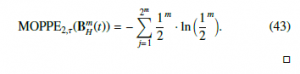
Order 2. In contrast to the previous sections, the behaviour of MOPPE on mfBm is obviously dependent on the number of variables m but remains independent of the delays τ.

Lemma 7.1 Let B^k_Hk (s) and B^l_Hl (t) for every k,l = 1,…,m conditionally independent, then it holds that

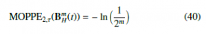
Proof. The independence from the delay τ follows directly from Definition 3.4 and the distribution of the univariate ordinal patterns of order d = 2 in (12). Let j ∈ {(0,1),(1,0)} be a univariate ordinal patterns of order d = 2. Let X_k = B^k_Hk (t) and X_l = B^l_Hl (t) for every k,l = 1,…,m conditionally independent, then the joint probability function satisfies

With (12) it is p_j = 1/2 for every j, so that the joint distribution of every m-fold combination of ordinal patterns j ∈ {(0,1),(1,0)} stays p_j^m. For the number of variables m, there exist 2^m multivariate ordinal patterns as combinations from univariate ordinal patterns so that

Orders greater than 2. For orders d = 3 and d = 4, the following theorem can be derived by considering joint probabilities of univariate ordinal pattern distributions introduced in Section 2.3.

Lemma 7.2 MOPPE(B^m_H(t)) of orders d = 3 and d = 4 are independent of all delays τ, but dependent on number of variables m, and monotonically dependent on the Hurst parameter H.

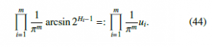
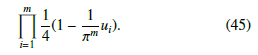
Proof. The independence from the delay τ follows directly from Definition 3.4 and the distribution of the univariate ordinal patterns or orders d = 3 or d = 4 in (13) or (15), respectively. As introduced in Section 2.3, the distribution of ordinal patterns of order d = 3 is twofold (see (14)). Therefore, let A = {(0,1,2),(2,1,0)} and B = {(0,2,1),(1,2,0),(1,0,2),(2,0,1)}. Since multivariate ordinal patterns are combinations of univariate ordinal patterns, in the following, we consider three cases where the ordinal patterns of all m variables are either from A, from B or from A and B. Again, let B^k_Hk (s) and B^l_Hl (t) be conditionally independent for each k,l = 1,…,m.

1. Let the univariate pattern a_i of the i-th variable be a_i ∈ A for all i = 1,…,m. Using (13) and (41) the joint distributions of all 2^m combinations of a₁,…,a_m ∈ A are given by

2. Let the univariate pattern b_i of the i-th variable be b_i ∈ B for all i = 1,…,m. Using (14) and (41) the joint distributions of all 4^m combinations of b₁,…,b_m ∈ B are given by

m = 3 in variation of Hurst parameters H_i = H_j for all i, j.

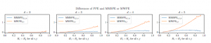
Figure 10: Differences of PPE and MMSPE or MWPE of different orders (from left to right) and fixed delay τ = 1 on simulations of mfBm with fixed number of variables

3. Let the univariate pattern c_i of the i-th variable be, where c₁,…,c_k ∈ A and c_k+1,…,c_m ∈ B. Then using (13), (14), and (41) the joint distributions of all 6^m − 4^m − 2^m remaining combinations c₁,…,c_m are given by

In particular, the joint distributions or the distributions of the multivariate ordinal patterns remain monotonically dependent on the Hurst parameter H after the monotonic transformations.

For order d = 4, formulas for joint distributions corresponding to multivariate ordinal patterns are derivable with (15) and (41) in the same way as for order d = 3.

For orders d > 4, no closed formulas for the distribution of ordinal patterns in fBm exist. Nevertheless, analogous behaviour of MOPPE of orders d > 4 can also be observed in this case, which we evaluate in an experimental setting in the next section.

7.2        Experimental Evaluation

In this experimental evaluation, we investigate the behaviour of MOPPE on mfBm in the variation of the Hurst parameter H and delay τ. Since the number of multivariate ordinal patterns depends on the number of variables m and thus also on MOPPE, we refrain from an experimental evaluation of different m, i.e., we assume m = 2 small for computational reasons. The experimental computations are based on the same simulations of mfBms as in Section 4.2 with the difference that in this experiment, we include more than one correlation parameter as MOPPE takes into account the interdependence of variables.

In Figure 11a we show the independence of MOPPE on mfBm from delay τ. For this, the number of variables is fixed to m = 2. Again, all green lines, i.e., for d = 2, are constant − ln(1/4) for each τ, confirming the independence of delay τ in (40). All other lines, i.e., for d > 2, are also the same for any τ, but monotonically dependent on the Hurst parameter H, i.e., for increasing Hurst parameter H the value of MOPPE decreases. The reason for the deviations of the values of MOPPE in Figure 11 with increasing Hurst parameter H is the same as in the previous Section 4. All in all, the experiment underpins our theoretical results from Theorem 7.1 and Theorem 7.2.

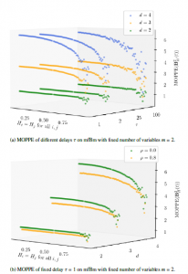
Figure 11: Experimental computations of MOPPE for different delays τ on mfBm with different correlations ρ = {0.0,0.8} in variation of its Hurst parameters H.

Although we have focused on independent variables in the theoretical part for simplicity as well as due to the lack of results in the literature, we examine the dependence on the correlations of variables in space in Figure 11b, since the definition of multivariate ordinal patterns involves the dependence on several variables. A high cross-covariance or correlation of the variables causes the behaviour of the individual variables (for different Hurst parameters) to converge. Another influences the behaviour of one variable, and so is the occurrence of the higher-order ordinal patterns that are dependent on the Hurst parameter. For the investigation of correlations using MOPPE, the delay or the number of variables are fixed to τ = 1 or m = 2, respectively. In Figure 11b, the yellow lines, corresponding to a correlation coefficient of 0.8, are constantly below the green lines corresponding to a correlation coefficient of 0.0. This reflects the fact that due to a higher correlation of the variables, there is a greater fit of the individual univariate ordinal pattern order in the multivariate combination, resulting in a smaller MOPPE value. Advantages are discussed in Section 8.

8. Comparison

Up to this point, we have examined the behaviour of numerous multivariate representations, namely pooled permutation entropy (PPE), multivariate multi-scale permutation entropy (MMSPE), multivariate weighted permutation entropy (MWPE), and multivariate ordinal pattern permutation entropy (MOPPE). In this section, we summarise both the differences and the similarities between the various representations. This leads to different possible applications as well as to different recommendations.

PPE can be understood as a canonical extension of univariate ordinal patterns to a multivariate variant that pools the univariate ordinal patterns over the variables. MMSPE and MWPE belong to the same family as PPE. They are all based on a pooled matrix while addressing different aspects of the time series and ordinal patterns, namely scaling and amplitudes. One advantage for these approaches is that, in contrast to MOPPE, they also allow univariate analyses on the individual variables within the algorithm. Figure 10 compares PPE with its extensions MMSPE and MWPE with different orders d = 1,…,5 from left to right. Since, as evaluated in the individual sections, all measures are independent of the delay and the number of variables, we set τ = 1 and m = 3. Similarly, MMSPE is independent of the scale parameter , so we set the scale factor  = 5. The left sub-figure shows the equality of PPE, MMSPE and MWPE for order d = 2, which again underpin (26), (30) and (31). Thus, scaling or weighting has no effect. The three right sub-figures in Figure 10 show the equality of PPE and MMSPE (blue lines) for orders d = 3,4,5. Similarly, they show a difference between PPE and MWPE as the orange lines increase in variation of increasing H, indicating a faster decrease of MWPE.

MOPPE can be understood as a canonical extension of univariate ordinal patterns to multivariate ordinal patterns by conceiving univariate patterns as multidimensional patterns in a matrix. The advantage of this approach lies in consideration of the interdependencies of several variables at a single time point. A disadvantage is the exponentially increasing number of possible ordinal patterns, which increase the complexity of the computation and result in a uniform distribution and thus maximum entropy for T  ∞. Furthermore, MOPPE considers the multivariate time series as a whole, i.e., not each variable individually, which means that an analysis of the individual variables using MOPPE within the algorithm is not possible, in contrast to PPE.

Differences in ρ_ij = {0.0,0.8} _1.50

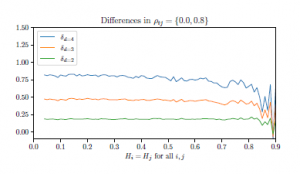
Figure 12: Differences of MOPPE values on mfBm with different correlations ρ_ij = {0.0,0.8} in variation of its Hurst parameter H.

Figure 12 visualises the differences of MOPPE values of different orders d = 2 (green), d = 3 (orange), and d = 4 (blue) and fixed delay τ on mfBm with fixed variable dimension m = 2 and different correlations ρ_ij = {0.0,0.8} in variation of its Hurst parameter H = (H₁, H₂), where H₁ = H₂. As the visualisation shows, the differences for any d ∈ {2,3,4} are almost constant for all Hurst parameters H. Increasing differences for increasing order d result from increasing maximum entropy values per order d.

The differences in the multivariate extensions of PE are important because they may be relevant to the use of different applications. In the field of inverse problems, the aim is to estimate the parameters, e.g., the Hurst parameter, of a generating dynamic system from observed realisations [36]. As all multivariate variants for orders d > 2 involve a direct relationship between the distribution of univariate ordinal patterns and the Hurst parameter H, PPE, MWPE and MOPPE are suitable candidates to solve the inverse problem regarding H. Given a realisation of mfBm, for example, the calculation of entropies that decrease as H increases can provide conclusions about the value of H. In addition to estimating H, MOPPE has the potential to uncover additional correlations by taking interdependencies into account, and it does so from one source. However, MOPPE is only practical for a small number of variables m. In machine learning, a high accuracy of the prediction depends not only on the model used but also on the representations of the data. Therefore, extracting good or expressive representations, also called features, from the data is essential. Especially in classification tasks, it is necessary to extract features that separate well [37]. In this case, MWPE may promise advantages over PPE because MWPE favours certain ordinal patterns (strictly rising and strictly falling) and thus decreases faster compared to PPE.

9. Conclusion and Future Work

Fractional Brownian motion (fBm) is usually used for modelling real-world applications with specific properties such as long-range dependence or self-similarity. Since many real-world applications also contain multivariate interdependencies between several variables, we focus on multivariate fractional Brownian motion (mfBm). This paper provides a comprehensive study of several multivariate measures that study the qualitative behaviour of multivariate fractional Brownian motion (mfBm), namely pooled permutation entropy (PPE), multivariate multi-scale permutation entropy (MMSPE), multivariate weighted permutation entropy (MWPE), and multivariate ordinal pattern permutation entropy (MOPPE). All measures are understood as multivariate extensions of univariate permutation entropy (PE), which is based on the distribution of ordinal patterns, i.e., on the ups and downs of different orders d ∈ N_>1. The main contributions of this paper are the extensions of the theoretical and experimental investigations of PPE, MMSPE and MWPE on mfBm in the original papers [1, 2] to additional orders d = 4 and d = 5. Furthermore, this paper provides a new study on the behaviour of MOPPE on mfBm, and for the first time, a comparison of all multivariate extensions considered.

Our theoretical and experimental analyses show the following results on the behaviour of PPE, MMSPE, MWPE and MOPPE on mfBm. For order d = 2, for all four cases the multivariate permutation entropy is constant − ln(1/2) regardless of number of variables, Hurst parameters, delays, scales, or weights (or − ln(1/2^m) in case of MOPPE). Because all measures are equal, in particular constant and independent of all parameters, no characteristics can be determined via these measures with order d = 2. Therefore, usage is not reasonable in applications. Since scaling does not change the structure of mfBm, MMSPE of any scale  is equal to PPE and analysis with MMSPE of higher orders d > 2 does not provide any additional insight than PPE.

However, for orders d > 2, the use of PPE, MWPE and MOPPE provide interesting insights and possible applications. The distribution of ordinal patterns, and thus also PPE, MWPE and MOPPE, are directly related to the Hurst parameter H. For example, considering the estimation of H is an inverse problem, PPE, MWPE and MOPPE can be used since they all depend monotonically on H, i.e., the entropy decreases as H increases. In contrast to PPE and MOPPE, MWPE is substantially influenced by strictly ascending and descending ordinal patterns. For this reason, MWPE decreases faster than PPE as H increases, providing more expressive representations that may promise better discriminability. Since multivariate ordinal patterns involve the dependence of several variables on mfBm, MOPPE is promising for estimating the Hurst parameter H and correlations from one hand, which the other measures cannot. To prove the exact theoretical relationship, conditional probabilities of univariate ordinal patterns must first be derived.

In the literature, there are additional approaches to multivariate permutation entropy determination, specifically Multivariate Permutation Entropy (MvPE), introduced in [30], or multivariate permutation entropy based on principal component analysis (MPEPCA), introduced in [33]. Since their application requires a prior transformation of mfBm and thus is not a canonical extension of the univariate definition, its study is not part of this work. Nevertheless, both have the potential to uncover (additional) structures in mfBm but are left for future work. In addition, the theoretical results of the measures investigated in this work motivate various potential applications, e.g., for estimating the Hurst parameter or as a feature in a learning task in the field of machine learning. Similarly, the application of these measures is of great interest not only in the context of mfBm but also for any real-world data set. Since this work focuses on the theoretic contexts, we leave concrete applications for future work.

1. M. Mohr, N. Finke, R. Mo¨ller, “On the Behaviour of Permutation Entropy on Fractional Brownian Motion in a Multivariate Setting,” in Proceedings of the Asia-Pacific Signal and Information Processing Association Annual Summit and Conference 2020 (APSIPA-ASC), 2020.
2. M. Mohr, F. Wilhelm, R. Mo¨ller, “On the Behaviour of Weighted Permutation Entropy on Fractional Brownian Motion in the Univariate and Multivariate Setting,” The International FLAIRS Conference Proceedings, 34, 2021, doi: 10.32473/flairs.v34i1.128464.
3. T. Konstantopoulos, S.-J. Lin, “Fractional Brownian Approximations of Queueing ing Networks,” in P. Glasserman, K. Sigman, D. D. Yao, editors, Stochastic Networks, 257–273, Springer New York, New York, NY, 1996.
4. R. J. Elliott, J. van der Hoek, “Fractional Brownian Motion and Financial Mod- elling,” in M. Kohlmann, S. Tang, editors, Mathematical Finance, 140–151, Birkha¨user Basel, 2001.
5. B. S. Nath, B. Mousumi, “Long Memory in Stock Returns: A Study of Emerg- ing Markets,” Iranian Journal of Management Studies, 5(2), 67–88, 2012.
6. F. Traversaro, F. O. Redelico, M. R. Risk, A. C. Frery, O. A. Rosso, “Bandt- Pompe symbolization dynamics for time series with tied values: A data-driven approach,” Chaos: An Interdisciplinary Journal of Nonlinear Science, 28(7), 2018, doi:10.1063/1.5022021.
7. J. Amigo´, Permutation Complexity in Dynamical Systems: Ordinal Patterns, Permutation Entropy and All That, Springer Series in Synergetics, Springer- Verlag, Berlin Heidelberg, 2010.
8. C. Bandt, F. Shiha, “Order Patterns in Time Series,” Journal of Time Series Analysis, 28(5), 646–665, 2007.
9. F. C. Morabito, D. Labate, F. La Foresta, A. Bramanti, G. Morabito, I. Pala- mara, “Multivariate Multi-Scale Permutation Entropy for Complexity Anal- ysis of Alzheimer’s Disease EEG,” Entropy, 14(7), 1186–1202, 2012, doi: 10.3390/e14071186.
10. B. Fadlallah, B. Chen, A. Keil, J. Principe, “Weighted-permutation entropy: A complexity measure for time series incorporating amplitude information,” Physical review. E, Statistical, nonlinear, and soft matter physics, 87, 022911, 2013, doi:10.1103/PhysRevE.87.022911.
11. M. Sinn, K. Keller, “Estimation of Ordinal Pattern Probabilities in Gaus- sian Processes with Stationary Increments,” Comput. Stat. Data Anal., 55(4), 1781–1790, 2011, doi:10.1016/j.csda.2010.11.009.
12. L. Zunino, D. G. Pe´rez, M. T. Mart´?n, M. Garavaglia, A. Plastino, O. A. Rosso, “Permutation entropy of fractional Brownian motion and fractional Gaussian noise,” Physics Letters A, 372(27), 4768–4774, 2008.
13. A. Da´valos, M. Jabloun, P. Ravier, O. Buttelli, “Theoretical Study of Multiscale Permutation Entropy on Finite-Length Fractional Gaussian Noise,” in 2018 26th European Signal Processing Conference (EUSIPCO), 1087–1091, 2018, doi:10.23919/EUSIPCO.2018.8553070, iSSN: 2076-1465.
14. L. A. Gil-Alana, “A fractional multivariate long memory model for the US and the Canadian real output,” Economics Letters, 81(3), 355–359, 2003, doi:10.1016/S0165-1765(03)00217-9.
15. S. Achard, D. S. Bassett, A. Meyer-Lindenberg, E. Bullmore, “Fractal connec- tivity of long-memory networks,” Physical Review E, 77(3), 2008.
16. B. B. Mandelbrot, J. R. Wallis, “Noah, Joseph, and Operational Hy- drology,” Water Resources Research, 4(5), 909–918, 1968, doi:10.1029/ WR004i005p00909.
17. G. Didier, V. Pipiras, “Integral representations and properties of operator fractional Brownian motions,” Bernoulli, 17(1), 1–33, 2011, doi:10.3150/ 10-BEJ259.
18. F. Lavancier, A. Philippe, D. Surgailis, “Covariance function of vector self- similar processes,” Statistics & Probability Letters, 79(23), 2415–2421, 2009, doi:10.1016/j.spl.2009.08.015.
19. G. Didier, V. Pipiras, “Integral representations and properties of operator frac- tional Brownian motions,” Bernoulli, 17(1), 1–33, 2011.
20. P.-O. Amblard, J.-F. Coeurjolly, F. Lavancier, A. Philippe, “Basic properties of the Multivariate Fractional Brownian Motion,” Se´minaires et congre`s, 28, 65–87, 2013.
21. P.-O. Amblard, J.-F. Coeurjolly, “Identification of the Multivariate Fractional Brownian Motion,” IEEE Transactions on Signal Processing, 59(11), 5152– 5168, 2011, doi:10.1109/TSP.2011.2162835.
22. B. Chiu, E. Keogh, S. Lonardi, “Probabilistic Discovery of Time Series Mo- tifs,” in Proceedings of the Ninth ACM SIGKDD International Conference on Knowledge Discovery and Data Mining, KDD ’03, 493–498, ACM, 2003.
23. C. Bandt, B. Pompe, “Permutation Entropy: A Natural Complexity Measure for Time Series,” Physical Review Letters, 88(17), 174102, 2002, publisher: American Physical Society.
24. K. Keller, T. Mangold, I. Stolz, J. Werner, “Permutation Entropy: New Ideas and Challenges,” Entropy, 19(3), 134, 2017, doi:10.3390/e19030134.
25. A. B. Piek, I. Stolz, K. Keller, “Algorithmics, Possibilities and Limits of Ordinal Pattern Based Entropies,” Entropy, 21(6), 547, 2019, doi:10.3390/e21060547.
26. K. Keller, S. Maksymenko, I. Stolz, “Entropy determination based on the ordi- nal structure of a dynamical system,” Discrete and Continuous Dynamical Sys- tems – Series B, 20(10), 3507–3524, 2015, doi:10.3934/dcdsb.2015.20.3507.
27. I. Stolz, K. Keller, “A General Symbolic Approach to Kolmogorov-Sinai En- tropy,” Entropy, 19(12), 675, 2017, doi:10.3390/e19120675.
28. M. Costa, A. L. Goldberger, C.-K. Peng, “Multiscale entropy analysis of complex physiologic time series,” Physical Review Letters, 89(6), 068102, 2002.
29. K. Keller, H. Lauffer, “Symbolic Analysis of High-Dimensional Time Series,” International Journal of Bifurcation and Chaos, 13(09), 2657–2668, 2003, doi:10.1142/S0218127403008168.
30. S. He, K. Sun, H. Wang, “Multivariate Permutation Entropy and Its Application for Complexity Analysis of Chaotic Systems,” Physica A: Statistical Mechanics and its Applications, 461, 812–823, 2016, doi:10.1016/j.physa.2016.06.012.
31. K. Keller, “Permutations and the Kolmogorov-Sinai Entropy,” Discrete & Continuous Dynamical Systems – A, 32(3), 891, 2012, doi:10.3934/dcds.2012.32.891.
32. A. Antoniouk, K. Keller, S. Maksymenko, “Kolmogorov-Sinai Entropy via Separation Properties of Order-Generated Sigma-Algebras,” Discrete and Con- tinuous Dynamical Systems, 34(5), 1793–1809, 2013, doi:10.3934/dcds.2014. 34.1793.
33. M. Mohr, F. Wilhelm, M. Hartwig, R. Mo¨ ller, K. Keller, “New Approaches in Ordinal Pattern Representations for Multivariate Time Series,” in Proceed- ings of the 33rd International Florida Artificial Intelligence Research Society Conference (FLAIRS-33), 124–129, AAAI Press, 2020.
34. Y. Rayan, Y. Mohammad, S. A. Ali, “Multidimensional Permutation Entropy for Constrained Motif Discovery,” in N. T. Nguyen, F. L. Gaol, T.-P. Hong, B. Trawin´ski, editors, Intelligent Information and Database Systems, Lecture Notes in Computer Science, 231–243, Springer International Publishing, Cham, 2019, doi:10.1007/978-3-030-14799-0 20.
35. N. Nicolaou, J. Georgiou, “The Use of Permutation Entropy to Characterize Sleep Electroencephalograms,” Clinical EEG and Neuroscience, 42(1), 24–28, 2011, doi:10.1177/155005941104200107.
36. B. D’Ambrogi-Ola, “Inverse Problem for Fractional Brownian Motion with Discrete Data,” 2009.
37. Y. Bengio, A. Courville, P. Vincent, “Representation Learning: A Review and New Perspectives,” IEEE Transactions on Pattern Analysis and Machine Intelligence, 35(8), 1798–1828, 2013, doi:10.1109/TPAMI.2013.50.

(Click Here)