1. Introduction

This paper is an extension of two works originally presented in KI 2021: Advances in Artificial Intelligence [1] and in AI 2021:

Advances in Artificial Intelligence – 34rd Australasian Joint Conference [2]. Both papers study the approximation of symmetries using an ordinal pattern symbolisation approach to prevent groundings in dynamic probabilistic relational models (DPRMs)^[1].

In order to cope with uncertainty and relational information of numerous objects over time, in many real-world applications, probabilistic temporal (also called dynamic) relational models (DPRMs) need often be employed [3]. Reasoning on large probabilistic models, like in data-driven decision making, often requires evaluating multiple scenarios by answering sets of queries, e.g., regarding the probability of events, probability distributions, or actions leading to a maximum expected utility (MEU). Further, reasoning on large respect, DPRMs, together with lifted inference approaches, provide an efficient formalism addressing this problem. DPRMs describe dependencies between objects, their attributes and their relations in a sparse manner. To encode uncertainty, DPRMs encode probability distributions by exploiting in-dependencies between random variables (randvars) using factor graphs. Factor graphs are combined with relational logic, using logical variables (logvars) as parameters for randvars to compactly represent sets of randvars that are considered indistinguishable (without further evidence). This technique is also known as lifting [5, 6]. A lifted representation of a probabilistic graphical model allows for a sparse representation to restrain state complexity and enables to decrease runtime complexity in inference.

To illustrate the potential of lifting, let us think of creating a probabilistic model for navigational route planning and congestion avoidance in dry-bulk shipping. Dry-bulk shipping is one of the most important forms of transportation as part of the global supply chain [7, 3]. Especially the last year 2020, which was marked by the coronavirus pandemic, shows the importance of good supply chain management. An important sub-challenge in supply chain management is congestion avoidance, which has been studied in research ever-since [8]-[10]. Setting up a probabilistic model to improve planning and to avoid congestion requires identifying features, such as demand for commodities and traffic volume, affecting any routing plans. Commodities are unevenly spread across the globe due to the different mineral resources of countries. In case of excessive demand, regions where the demanded commodities are mined and supplied are excessively visited for shipping, resulting in congestion in those regions. If such a model includes only a few objects, here regions from which commodities are transported, the model might still be considerably small, but once including more regions to capture the whole market, i.e., with an increasing domain size, the complexity of the model increases. However, with an increase in complexity due to an increase in the domain size also the likelihood of keeping redundant information within the model increases. For example, in the application of route planning, multiple regions may exist that are similar in terms of features of the model. Intuitive examples are regions offering the same commodities, i.e., regions with similar mineral resources.

Lifting exactly exploits that existence: Regions which are symmetrical with respect to the features used in the model can be treated by one representative for a group of symmetrical objects to obtain a sparser representation of the model. Further, by exploiting those occurrences, reasoning in lifted representations has no longer a complexity exponential in the number of objects represented by the model, here regions, but is limited to the number of objects with asymmetries only [11, 12]. More specifically, symmetries across objects of a models domain, i.e., objects over randvars of the same type, are exploited by means of performing calculations in inference only once for groups of similarly behaving objects, instead of performing the same calculations over and over again for all objects individually. The principle of lifting applies not only to logistics but also to many other areas like politics, healthcare, or finance – just to name a few.

DPRMs encode a temporal dimension and can be used in any online scenario, i.e., new knowledge is on the fly encoded to enable for continuous query answering without relearning the model. In existing research, it is assumed that lifted graphical models already contain symmetries, i.e., simply speaking, a model is setup so that all objects behave according to the same probability distribution. New knowledge is then incorporated in the model with new observations for each object. Observations are encoded within the model as realisations of randvars, resulting in a split off from a symmetrical consideration, called grounding. Of course, if the same observation is made for multiple objects, those objects are split off together and continue to be treated as a group. Over time, models dissolve into groups of symmetrically behaving objects, i.e., symmetries are implicitly exploited. Note that in the worst case, the models are split in such way that all objects are treated individually, i.e., no symmetries are available in the model so that lifted inference can no longer be applied and all its advantages disappear.

To the best of our knowledge, existing research has not yet focused on constructing symmetries in advance instead of deriving symmetries implicitly. Constructing symmetries in advance has benefits in application and results from the characteristics of real-world applications:

• Certain information about objects of the model may not be available at runtime but only become known downstream. In such cases it is beneficial to infer information according to the open-world assumption from the behaviour of other object which tend to behave similar, i.e., applying an intrinsic default. On the one hand wrong information can be introduced in the model, but on the other it is likely that objects continue to behave the same as per other objects.
• Symmetrical objects can behave the same in the long term, but may deviate for shorter periods of time. Even already small deviations lead to groundings in the model, which, if prevented, introduce a small error in the model, but which also is negligible in the long term.

In both cases a model grounds, which must be prevented in order to keep reasoning in polynomial time. We construct groups of objects with similar behaviour, which we denote as symmetry clusters, through a symbolisation scheme to approximate temporal symmetries, i.e., objects that tend to behave the same over time. Using the symmetry clusters, it is possible to selectively prevent groundings, which helps to retain a lifted representation.

This work contributes with a summary on approximating model symmetries in DPRMs based on multivariate ordinal pattern symbolisation and clustering to obtain groups of objects with approximately similar behaviour. Behaviour is derived from the realisations of randvars, which generate either a univariate or multivariate time series depending on the number of interdependent randvars in the model. In the first original conference paper [1], we present multivariate ordinal pattern symbolisation for symmetry approximation (MOP₄SA) for the univariate case and introduce symmetry approximation for preventing groundings (SA₄PG) as an algorithm to prevent groundings in inference a priori using the learned entity symmetry clusters. In the second original conference paper [2], we extend MOP₄SA to the multivariate case and motivate the determination of related structural changes and periodicities in symmetry structures. Further, this work contributes with an extension of original works in [1] and [2] by

• a comprehensive review of MOP₄SA and SA₄PG with additional applications from dry-bulk shipping,
• a complement of the existing theoretical and experimental investigations of MOP₄SA and SA₄PG in the variation of its parameters, i.e., we fill in the gaps by investigating different orders and delays for ordinal patterns while also examining different thresholds in the symmetry approximation with respect to the introduced error in inference, and
• a new approach named MOP₄SCD to detect changes in symmetry structures based on a models similarity graph, an intermediate step of MOP₄SA, to re-learn symmetries on demand.

Together MOP₄SA, SA₄PG and multivariate ordinal pattern symbolisation for symmetry change detection (MOP₄SCD) combine into a rich toolset to identify model symmetries as part of the model construction process, use those symmetries to maintain a lifted representation by preventing groundings a priori and detect changes in model symmetries after the model construction process.

This paper is structured as follows. After presenting preliminaries on DPRMs in Section 2, we continue in Section 3 with an review on how to retain lifted solutions through approximation and its relation to time series analysis and common approaches to determine and approximate similarities in that domain. In the following, we recapitulate MOP₄SA, an approach that encodes entity behaviour through ordinal pattern symbolisation in Section 4.1 and summarise approximating entity symmetries based on the symbolisation in Section 4.2. In Section 5 we outline SA₄PG and elaborate how to prevent groundings in DPRMs a priori with the help of entity symmetry clusters. In Section 6 we evaluate both MOP₄SA and SA₄PG in a shipping application and provide a detailed discussion on its various parameters and its effect on the accuracy in inference. In Section 7 we introduce a new approach to detect changes in symmetry structures to uncover points in time at which relearning of symmetry clusters becomes beneficial. In Section 9 we conclude with future work.

2. Background

In the following, we recapitulate DPRMs [5] in context of an example in logistics, specifically dry-bulk shipping. Dry-bulk shipping is one of the most important forms of transportation as part of the global supply chain [7, 3]. Especially the last year 2020, which was marked by the coronavirus pandemic, showed the importance of good supply chain management. The global supply chain was heavily affected as a result of required lock-downs all over the world, which has led to disruptions and significant delays in delivery. An important sub-challenge in supply chain management is to avoid congestion in regions/zones in which cargo is loaded, i.e., making sure that vessels arrive when those regions are not blocked by too many other vessels being anchored up in same. Congestion avoidance has always been an important topic in research [8]-[10]. As follows, we setup a DPRM to infer idle times related to global supply for commodities. As such, we formally define DPRMs and elaborate on sparse representations and more efficient inference by exploiting symmetries to enable for faster decision making.

2.1. A Formal Model on Congestion in Shipping

We setup a simplified DPRM to model congestion resulting in idle times in different regions/zones across the globe. To infer idle times in certain zones, we use freight rates, a fee per ton, which is paid for the transportation of cargoes and differs across zones, as a driver for operators to plan their vessel movements. E.g., an increase in idle time in a zone can be caused by a high freight rate in that same zone, resulting in an higher interest for sending vessels due to the potential to gain higher profits due to high freight rates. Of course, even though freight rates might be higher, not every vessel operator will be able to conclude business in zones which are over-crowed or have higher waiting times increasing costs for lay time. Hence, to describe the interaction between waiting times and freight rates, the idle condition and freight rates in a zone can be represented by one randvar. Freight rates itself are driven by the supply of commodities in zones represented by another randvar. Since idle conditions, freight rates and supply can be similar in multiple zones, we can develop a much smaller model and combine all randvars into one and parameterise these with a logvar to represent the set of all zones respectively. In this example one zone from the set of all zones is referred to as an object or entity, which we use interchangeably moving forward. Such a parameterised random variable is referred to as PRV for short.

Definition 2.1 (PRV) Let R be a set of randvar names, L a set of logvar names, Φ a set of factor names, and D a set of entities. All sets are finite. Each logvar L has a domain D(L) ⊆ D. A constraint is a tuple (X,C_X) of a sequence of logvars X = (X₁,…, X_n) and a set C_X . A PRV A(L₁,…, L_n),n ≥ 0 is a construct of a randvar name A ∈ R combined with logvars L₁,…, L_n ∈ L. Then, the term R(A) denotes the (range) values of a PRV A. Further, the term lv(P) refers to the logvars and rv(P) to the randvars in some element P. The term gr(P_|C) denotes the set of instances of P with all logvars in P grounded w.r.t. constraint C.

The idea behind PRVs is to enable for combining objects with similar behaviour in a single randvar to come up with a sparse representation, introducing a technique called lifting. To model the interaction between idle times, freight rates and supply in zones across the globe, we use randvars Idle, Supply and Rate parameterised with a logvar Z representing zones, building PRVs Idle(Z), Supply(Z) and Rate(Z). The domain of Z is {z₀,z₁,…,z_n} and range values for all PRVs are {high,medium,low}^[2]. A constraint C = (Z, {z₁,z₂}) for Z allows to restrict Z to a subset of its domain, such as here to z₁ and z₂. Using this constraint, the expression gr(Idle(Z)_|C) evaluates to {Idle(z₁), Idle(z₂)}. To represent independent relations, PRVs are linked by a parametric factor (parfactor) to compactly encode the full joint distribution of the DPRM.

Definition 2.2 (Parfactor) We denote a parfactor g by φ(A)_|C with A = (A¹,…, Aⁿ) a sequence of PRVs, φ : ×ⁿ_i=1R(Aⁱ) →7 R⁺ a function with name φ ∈ Φ, and C a constraint on the logvars of A. A PRV A or logvar L under constraint C is given by A_|C or L_|C, respectively. An instance is a grounding of P, substituting the logvars in P with a set of entities from the constraints in P. A parameterized model PRM G is a set of parfactors {gⁱ}ⁿ_i=1, representing the full joint distribution P_G = _Z^{1 Q}_{f ∈gr(G)} f, where Z is a normalizing constant.

All PRVs are dependent on each other and therefore are combined through one parfactor g¹ = φ¹(Idle(Z),Rate(Z),Supply(Z)), (1)

which denotes their joint probability distribution. We omit the concrete mappings of potentials to range values of φ¹. To encode temporal behaviour, DPRMs follow the same idea as dynamic Bayesian networks (DBNs) with an initial model and a temporal copy pattern to describe model changes over time. DPRMs model a stationary process, i.e., changes from one time step to the next follow the same distribution.

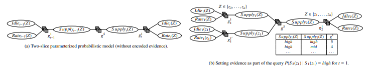Figure 1: Graphical representation of a slice of a dynamic probabilistic graphical model illustration how to encode evidence.

Definition 2.3 (DPRM) A DPRM is a pair of PRMs (G₀,G_→) where G₀ is a PRM representing the first time step and G_→ is a two-slice temporal parameterized model representing A_t−1 and A_t where A_π is a set of PRVs from time slice π. An inter-slice parfactor φ(A)_|C has arguments A under constraint C containing PRVs from both A_t−1 and A_t, encoding transitioning from time step t − 1 to t. A DPRM (G₀,G_→) represents the full joint distribution P_(G0,G→),_T by unrolling the DPRM for T time steps, forming a PRM as defined above.

Figure 1a shows the final DPRM. Variable nodes (ellipses) correspond to PRVs, factor nodes (boxes) to parfactors. Edges between factor and variable nodes denote relations between PRVs, encoded in parfactors. The parfactor g^S denotes a so-called inter-slice parfactor that separates the past from the present. The submodel on the left and on the right of this inter-slice parfactor are duplicates of each other, with the one on the left referring to time step t − 1 and the one on the right to time step t. Parfactors reference time-indexed PRVs, namely Idle_t(Z), Rate_t(Z) and Supply_t(Z).

2.2. Query Answering under Evidence

Given a DPRM, one can ask queries for probability distributions or the probability of an event given evidence.

Definition 2.4 (Queries) Given a DPRM (G₀,G_→), a ground PRV

Q_t, and evidence E_0:t = {{E_s,i = e_s,i} (set of events for time steps 0 to t), the term P(Q_π | E_0:t), π ∈ {0,…,T}, t ≤ T, denotes a

query w.r.t. P(G0,G→),T.

In context of the shipping application, an example query for time step t = 2, such as P(Supply₂(z₁) | Supply₁(z₁) = high), which asks for the probability distribution of supply at time step t = 2 in a certain zone z₁, given that in the previous time step t = 1 the supply was high, contains an observation Supply₁(z₁) = high as evidence. Sets of parfactors encode evidence, one parfactor for each subset of evidence concerning one PRV with the same observation.

Definition 2.5 (Encoding Evidence) A parfactor g_e = φ_e(E(X))_|Ce encodes evidence for a set of events {E(x_i) = o}ⁿ_i=1 of a PRV E(X). The function φ_e maps the value o to 1 and the remaining range values of E(X) to 0. Constraint C_e encodes the observed groundings x_i of E(X), i.e., C_e = (X, {x_i}ⁿ_i=1).

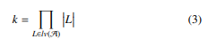
Figure 1b depicts how evidence for t = 1, i.e., to the left of the interslice parfactor g^S , is set within the lifted model.

Evidence is encoded in parfactors0 g¹₁⁰ by duplicating the original parfactor g¹₁ and using g¹₁ to encode evidence and g¹₁ to represent all sets of entities that are still considered indistinguishable. Each parfactor represents a different set of entities bounded by the use of constraints, i.e., limiting the domain for the evidence parfactor g¹₁⁰ to {z₁} and the domain for the original parfactor g¹₁ to D(Z) \ {z₁}. The parfactor that encodes evidence is adjusted such that all range value combinations in the parfactors distribution φ for Supply₁(z₁) , high are dropped. Groundings in one time step are transferred to next time steps, i.e., also apply to further time steps, which we discuss as follows.

2.3. The Problem of Model Splits in Lifted Variable Elimination for Inference

As shown in Fig. 1b, evidence leads to groundings in the lifted model. Those model splits are carried over in message passing over time when performing query answering, i.e., in inference. Answering queries, e.g., asking for the probability of an event, results in joining dependent PRVs, or more specifically, joining those parfactors with overlapping PRVs. Figure 1b shows a sample of the probability distribution for the interslice parfactor g^S which separates time steps t − 1 and t. Answering the query

P(Supply₂(z₁) | Supply₁(z₁) = high as per the example in Section 2.1 to obtain the probability distribution over supply in time step t = 2, requires to multiply parfactors g¹₁⁰ with the interslice parfactor g^S and the parfactor g¹₂. However, since in time step t = 1 a grounding for z₁ exists, the grounding is carried over to the following time step t = 2 as the PRV Supply₁(z₁) is connected to the following time step via the interslice parfactor g^S . Therefore, evidence, here Supply₁(z₁) = high, is also set within g^S dropping all range values for Supply₁(z₁) , high. This step is necessary to obtain an exact result in inference. For any other queries, this evidence is carried over to all future time steps, accordingly. Thus, under evidence a model G_t = {gⁱ_t}ⁿ_i=1 at time step t is split w.r.t. its parfactors such that its structure remains

with k ∈ N⁺. Every parfactor gⁱ_t can have up to k ∈ N⁺ splits gⁱ_t^,j = φⁱ_t^,j(Aⁱ)_|Ci_,j , where 1 ≤ j ≤ k and Aⁱ is a sequence of the same PRVs but with different constraint C^i,j and varying functions φⁱ_t^,j due to evidence. Note that moving forward we use the terms parfactor split or parfactor group interchangeably.

In our example, the model is only splitted with regards to evidence for the entity z₁. All other entities are still considered to be indistinguishable, i.e., lifted variable elimination (LVE) can still exploit symmetries for those instances. To do so, lifted query answering is done by eliminating PRVs, which are not part of the query, by so called lifted summing out. Basically, variable elimination is computed for one instance and exponentiated to the number of isomorphic instances represented. Gehrke et al. [5] introduce the lifted dynamic junction tree (LDJT) algorithm for query answering on DPRMs, which uses LVE [6, 13] as a subroutine during its calculations. For a full specification of LDJT, we recommend to read on in [5]. In the worst case a model is fully grounded, i.e., a model as defined in Eq. (12) contains

splits for every parfactor gⁱ_t = φⁱ_t(A)_|Ci such that each object l ∈ L is in its own parfactor split. The problem of model splits, i.e., groundings, can generally be traced back to two aspects. Groundings arise from

• partial evidence or unknown evidence, i.e., certain information about objects of the model may not be available at runtime and either never or only become known downstream, which we denote as unknown inequality, or
• from different observations for two ore more objects, i.e., objects show different behaviour requiring to consider those individually moving forward, which we denote as known inequality.

Once the model is split, those splits are carried forward over time, potentially leading to a fully ground model. By doing so, the model remains exact as new knowledge (in form of observations) is incorporated into the model in all details. Over time, however, distinguishable entities might align and can be considered as one again (in case of known inequality) or entities might have ever since behaved similarly without knowing due to less frequent evidence (in case of unknown inequality). To retain a lifted representation the field of approximate inference, i.e., approximating symmetries, has emerged in research.

3. Related Work on Retaining Lifted Solutions Through Approximation and the Connection to Time Series Analysis

Lifted inference approaches suffer under the dynamics of the real world, mostly due to asymmetric or partial evidence. Handling asymmetries is one of the major challenges in lifted inference and crucial for its effectiveness [14, 15]. To address that problem, approximating symmetries has emerged in related research that we discuss in the following.

3.1. Approximate Lifted Models

For static (non-temporal) models, Singla et al. [16] propose to approximate model symmetries as part of the lifted network construction process. They perform Lifted Belief Propagation (LBP) [17], which constructs a lifted network, and apply Belief Propagation (BP) to it. The lifted network is constructed by simulating message passing and identifying nodes sending the same message. To approximate the lifted network, message passing is stopped at an earlier iteration to obtain an approximate instance. Ahmadi et al. [18] also approximate symmetries using LBP, but propose piece-wise learning [19] of the lifted network. That means that the entire model is divided into smaller parts which are trained independently and then combined afterwards. In this way, evidence only influences the factors in each part, yielding a more liftable model. Besides approaches using LBP, Venugopal and Gogate [20] propose evidence-based clustering to determine similar groundings in an Markov Logic Network (MLN). They measure the similarity between groundings and replace all similar groundings with their cluster centre to obtain a domain-reduced approximation. Since the model becomes smaller, also inference in the approximated lifted MLN is also much faster. Van den Broek and Darwiche [15] propose so-called over-symmetric evidence approximation by performing low-rank boolean matrix factorisation (BMF) [21] on MLNs. They show, that for evidence with high boolean rank, a low-rank approximate BMF can be found. Simply put, finding a low-rank BMF corresponds to removing noise and redundant information from the data, yielding a more compact representation, which is more efficient as more symmetries are preserved. As with any existing approach to symmetry approximation, inference is performed on the symmetrised model, ignoring the introduction of potentially spurious marginals in the model. Van den Broeck and Niepert [12] propose a general framework that provides improved probability estimates for an approximate model. Here, a new proposal distribution is computed using the Metropolis-Hasting algorithm [22, 23] on the symmetrised model to improve the distribution of the approximate model. Their approach can be combined with any existing approaches to approximate model symmetries.

Still, most of the existing research is based on static models and requires to get evidence in advance. However, the problem of asymmetric evidence is particularly noticeable in temporal models, and even more so in an online setting, since performing the symmetry approximation as part of the lifted network construction process is not feasible [24]. That means that it is necessary to construct a lifted temporal model once and to encode evidence as it comes in over time. Continuous relearning, i.e., reconstructing the lifted temporal model before performing query answering, is too costly. For temporal models Gehrke et al. [25] propose to create a new lifted representation by merging groundings introduced over time. They perform clustering to group sub-models and perform statistical significance checks to test if groups can be merged.

In comparison to that and to the best of our knowledge, no-one has focused on preventing groundings before they even occur. To this end, we propose to learn entity behaviour in time and cluster entities that behave approximately similar in the long run and use them to accept or reject incoming evidence to prevent the model from grounding. Clustering entity behaviour requires approaches which find symmetries in entity behaviour, i.e., clustering entities which tend to behave the same according to observations made for them. As observations collected over time result in a time series our problem comes down to identify symmetries across time series.

3.2. From DPRMs to Time Series

In a DPRM, (real-valued) random variables observed over time are considered as time series. Let Ω be a set containing all possible states of the dynamical system, also called state space. Events are taken from a σ-algebra A on Ω. Then (Ω, A) is a measurable space. A sequence of random variables, all defined on the same probability space (Ω, A,µ), is called a stochastic process. For real-valued random variables, a stochastic process is a function

where X(ω,t) := X_t(w) depending on both, coincidence and time. Note that in the most simple case Ω matches with R and X with the identity map. Then the observations are directly related to iterates of some ω, i.e., there is no latency, and the X itself is redundant. Over time, the individual variables X_t(ω) of this stochastic process are observed, so-called realisations. The sequence of realisations is called time series. With the formalism from above and fixing of some ω ∈ Ω, a time series is given by

In the case x_t ∈ R the time series is called univariate, while in the case x_t ∈ R^m it is called multivariate. Note that for stochastic processes we use the capitalisation (X(t))_t∈N, while for observations, i.e., paths or time series, we use the small notation (x(t))_t∈N. In summary, evidence in a DPRM encoding stochastic processes (X(t))_t∈N forms a time series (x_t)_t∈N that is the subject of further consideration.

3.3. Symmetry Approximation in Time Series

In time series analysis, the notion of similarity, known as symmetry in DPRMs, has often been discussed in the literature [26]-[28]. In general, approaches for finding similarities in a set of time series are either (a) value-based, or (b) symbol-based. Value-based approaches compare the observed values of time series. By comparing the value of each point x_t, t = 1,…,T in a time series X with the values of each other point y_t0, t⁰ = 1,…,T ⁰ in another time series Y (warping), they are able to include shifts and frequencies. Popular algorithms such as dynamic time warping (DTW) [29] or matrix profile [30] are discussed, e.g., in [28]. As DPRMs can encode interdependencies between multiple variables, respective multivariate procedures should be used to assess similarities. The first dependent multivariate dynamic time warping (DMDTW) approach is reported by Petitjean et al. [31], in which the authors treat a multivariate time series with all its m interdependencies as a whole. The flexibility of warping in value-based approaches leads to a high computational effort and is therefore unusable for large amounts of data. Although there are several extensions to improve runtime [32] by limiting the warping path or reducing the number of data points, e.g., FastDTW [32] or PrunedDTW [33], the use of dimensionality reduction is inevitable in context of DPRMs. For dimensionality reduction, symbol-based approaches encode the time series observations as sequences of symbolic abstractions that match with the shape or structure of the time series. Since DPRMs encode discrete values, depending on the degree for discretisation, symbol-based approaches are preferred as they allow for discretisation directly. As far as research is concerned, there are two general ways of symbolisation. On the one hand, classical symbolisation partitions the data range according to specified mapping rules in order to encode a numerical time series into a sequence of discrete symbols. A corresponding and well-know algorithm is Symbolic Aggregate ApproXimation (SAX) introduced by Chiu et al. [34]. On the other hand, as introduced by Bandt and Pompe [35] ordinal pattern symbolisation encodes the total order between two or more neighbours (x < y or x > y) into so-called ordinal symbols ((0,1) or (1,0)). Mohr et al. [36] extend univariate ordinal patterns to the multivariate case, taking into account not only the dependencies of neighbouring values over time, but also the dependencies between spatial variables in a time series.

Specifically here, an ordinal approach has notable advantages in application: (i) The method is conceptionally simple, (ii) the ordinal approach supports robust and fast implementations [37, 38], and (iii) compared to classical symbolisation approaches such as SAX, it allows an easier estimation of a good symbolisation scheme [39, 40]. In the following, we introduce ordinal pattern symbolisation to classify similar entity behaviour.

4. Multivariate Ordinal Pattern for Symmetry Approximation (MOP₄SA)

In this section we recapitulate MOP₄SA, an approach for the approximation of symmetries over entities in the lifted model. MOP₄SA consists of two main steps, which is (a) encoding entity model behaviour through an ordinal pattern symbolisation approach, followed by (b) clustering entities with a similar symbolisation scheme to determine groups of entities with approximately similar behaviour. We have introduced MOP₄SA in [1] for the univariate case and extended same in [2] to the multivariate case.

4.1. Encoding Entity Behavior through Ordinal Pattern Symbolisation

As mentioned in Section 3.3, approximating entity behaviour corresponds to finding symmetries in time series.

4.1.1     Gathering Evidence

To find symmetries in (multivariate) time series, we use evidence which encode model entity behaviour w.r.t. a certain context, i.e., w.r.t. a parfactor. In particular, this means: Every time-index PRV P_t(X) represents multiple entities x₀,…, x_n of the same type at a specific point in time t. That is, for a PRV Supply_t(Z), zones z₀,…,z_n are represented by a logvar Z with domain D(Z) and size |D(Z)|. Note that a PRV can be parameterised with more than one logvar, but for the sake of simplicity we introduce our approach using PRVs with only one logvar throughout this paper. Symmetry detection for m-logvar PRVs works similarly to one-logvar PRVs, with the difference, that in symmetry detection, entity pairs, i.e., m-tuples, are used. As an example, for any 2-logvar PRV P_t(X,Y), an entity pair is a 2-tuple (x₁,y₁) with x₁ ∈ D(X) and y₁ ∈ D(Y).

A DPRM, as introduced in Section 2.1, encodes temporal data by unrolling a DPRM while observing evidence for the models PRVs, e.g., the PRV Supply_t(Z) encodes supply at time t in various zones Z on the globe. In addition, a DPRM exploits (conditional) independencies between randvars by encoding interdependencies in parfactors. As such, parfactors describe interdependent data through its linked PRVs, e.g., the correlation between supply Supply_t(Z), idle times Idle_t(Z) and freight rates Rate_t(Z) within a common zone Z encoded by the parfactor g¹_t . For each entity z_i ∈ D(Z) from the PRVs P = {Supply_t(Z), Idle_t(Z) and Rate_t(Z)} observations are made over time, i.e., a time series ((x_tⁱ)^m_i=1)^T_t=1 with x_tⁱ ∈ R(Pⁱ) is generated. In this work, the time series is to be assumed multivariate, containing interdependent variables, i.e., m > 1. Note that in [1] we consider the case m = 1. Having |D(Z)| entities in Z, we consider |D(Z)| samples of multivariate time series

(Supply_t(z_j), Idle_t(z_j),Rate_t(z_j)) for every z_j ∈ D(Z) in time t ∈ {1,…,T}. As such, a multivariate time series is defined for several PRVs linked in a parfactor, while a univariate time series is defined for a single PRV. Identification of symmetrical entity behaviour is done on a sets of (multivariate) time series, i.e., across different (multivariate) time series that are observed for every entity individually.

4.1.2     Multivariate Ordinal Pattern (MOP) Symbolisation

To encode the behaviour of a time series, we use ordinal pattern symbolisation based on works from Bandt and Pompe [35]. For this, let X_t ∈ R^m×T be a (multivariate) time series and X_t ∈ R^m×T×n be the reference database of n ∈ N (multivariate) time series. In case of m = 1, the time series is univariate. For a better understanding, we start with univariate ordinal patterns that encode the up and downs in a time series by the total order between two or more neighbours. The encoding gives a good abstraction, an approximation, of the overall behaviour or generating process. Univariate ordinal patterns are formally defined as follows.

Definition 4.1 (Univariate Ordinal Pattern) A vector (x₁,…, x_d) ∈

R^d has ordinal pattern (r₁,…,r_d)                 ∈ N^d of order d              ∈ N if

xr1 ≥ … ≥ xrd and rl−1 > rl in the case xrl−1 = xrl .

Figure 2 shows all possible ordinal patterns of order d = 3 of a vector (x₁, x₂, x₃) ∈ R³.

Figure 2: All d! possible univariate ordinal patterns of order d = 3.

For a multivariate time series ((x_tⁱ)^m_i=1)^T_t=1, each variable xⁱ for i ∈ 1,…,m depends not only on its past values but also has some dependency on other variables. To establish a total order between two time points (^x_tⁱ) and (^x_tⁱ₊₁)^m_i=1 with m variables is only possible if x_tⁱ > x_tⁱ₊₁ or x_tⁱ  for all i ∈ 1,…,m. Therefore, there is no trivial generalisation to the multivariate case. An intuitive idea, based on some theoretical discussion in [41, 42] and introduced in [36], is to store univariate ordinal patterns of all variables at a time point t together into a symbol.

Definition 4.2 (Multivariate Ordinal Pattern) A                        matrix

(x₁,…, x_d) ∈ R^m×d has multivariate ordinal pattern (MOP) of order d ∈ N

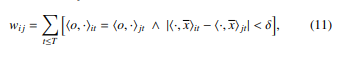
For m = 1 the multivariate case matches with the univariate case in Definition 4.1. Figure 3 shows all (d!)^m possible multivariate ordinal patterns (MOPs) of order d = 3 and number of variables m = 2.

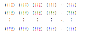Figure 3: All (d!)^m possible multivariate ordinal patterns of order d = 3 with m = 2 variables.

The number of possible MOPs d! increases exponentially with the number of variables m, i.e., (d!)^m. Therefore, if d and m are too large, depending on the application, each pattern occurs only rarely or some not at all, resulting in a uniform distribution of ordinal patterns [36]. This has the consequence that subsequent learning procedures can fail. Nevertheless, for a small order d and sufficiently large T the use of MOPs can lead to higher accuracy in learning tasks, e.g., classification [36] because they incorporate interdependence of the spatial variables in the multivariate time series.

To symbolise a multivariate time series X_t ∈ R^m×T each pattern is identified with exactly one of the ordinal pattern symbols o = 1,2,…,d!, before each point t ∈ {d,…,T} is assigned its ordinal pattern symbol of order d  T. The order d is chosen much smaller than the length T of the time series to look at small windows in a time series and their distributions of up and down movements. To assess long-term trends, delayed behaviour is of interest, showing various details of the structure of the time series. The time delay τ ∈ N_>0 is the delay between successive points in the symbol sequences.

4.1.3     MOP Symbolisation with Data Range Dependence

We assume that for each time step t = τ(d − 1) + 1,…,T of a multivariate time series ((x_tⁱ), MOP is determined as described in Section 4.1.2. Ordinal patterns are well suited to characterise an overall behaviour of time series, in particular their application independent of the data range. In some applications, however, the dependence on the data range can be also relevant, i.e., time series can be similar in terms of their ordinals patterns, but differ considering their y-intercept. In other words, transforming a sequence

as y = x + c, where c ∈ R is a constant, should change y’s similarity to other sequences, although the shape is the same. To address the dependence on the data range, we use the arithmetic mean

of the multivariate time series’ values corresponding to the ordinal pattern, where x_{i,t−(k−1)τ} is min-max normalised, as an additional characteristic or feature of behaviour. If one of the variables changes its behaviour significantly along the intercept, the arithmetic mean uncovers this. There are still other features that can be relevant. For simplicity, we only determine ordinal patterns and their means for each parfactor g¹ with, e.g., PRVs (Supply_t(Z), Idle_t(Z), Rate_t(Z)), yielding a new data representation

where ho, ·i_tj ∈ X⁰ represents the MOP and h·, xi_tj ∈ X⁰ represents the corresponding mean x^d_t ^,τ for entity z_j at time step t. The order d and delay τ are passed in from the outside and might depend on, e.g., the frequency of the data, to capture the long-term behaviour.

4.2. Clustering Entities with Similar Symbolisation Scheme

After encoding the behaviour of the entities through ordinal pattern symbolisation, we identify similar entities using clustering. For this purpose, based on the derived symbolisation representation in Eq. (10), we create a similarity graph indicating the similarities based on a distance measure between entity pairs.

4.2.1     Creating a Similarity Graph

Entity similarity is measured per parfactor, i.e., per multivariate time series, separately. Therefore, multiple similarity graphs, more specifically one per parfactor, are constructed. A similarity graph for a parfactor g¹_t connecting the PRVs Supply_t(Z), Idle_t(Z) and Rate_t(Z) contains one node for each entity z ∈ D(Z) observed in form of multivariate time series. The edges of the similarity graph represent the similarity between two nodes, or more precisely, how closely related two entities of the model are. To measure similarity, we use the symbolic representation X⁰, which contains tuples of multivariate ordinal numbers and mean values that describe the behaviour of an entity. The similarity of two entities z_i and z_j is given by counts w_ij of equal behaviours, i.e.,

where [x] = 1 if x and, 0 otherwise. As an auxiliary structure, we use a square matrix W ∈ N^{|D(Z)|×|D(Z)|}, where each w_ij ∈ W describes the similarity between entities z_i and z_j by simple counts of equal behaviour over time t ∈ T. Simply put, one counts the time steps t at which both multivariate time series of z_i and z_j have the same MOP and the absolute difference of the mean values of the corresponding MOPs is smaller than δ > 0. Finally, as shown in Figure 4b the counts w_ij correspond to the weights of edges in the similarity graph W, where zero indicates no similarity between two entities, while the larger the count, the more similar two entities are.

 

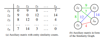Figure 4: (a) Auxiliary matrix and (b) similarity graph.

Approximating symmetries based on the similarity graph leaves us with a classical clustering problem. That means, clustering entities into groups of entities showing enough similarities or leaving others independent if those are too different.

4.2.2      Derive Entity Similarity Clusters

Theoretically, any clustering algorithm can be applied on top of the similarity graph. Each weight in the similarity matrix, or each edge weight between an an entity pair, denotes the similarity between two entities, i.e., the higher the count, the more similar the two entities are to each other. Since this contribution focuses on identifying symmetries in temporal environments, we leave the introduction of a specific clustering algorithm out here, and compare two different ones, specifically Spectral Clustering and Density-Based Spatial Clustering of Applications with Noise (DBSCAN), for the use in MOP₄SA as part of the evaluation in Section 6. After any clustering algorithm is run, we are left with n clusters of entities for each parfactor. Formally, a symmetry cluster is defined as follows.

Definition 4.3 (Symmetry Cluster) For a parfactor g_i ∈ G_t with G_t being the PRM at timestep t and g_i = φ(A)_|C containing a sequence of PRVs A = (A¹,…, Aⁿ), a symmetry cluster S ⁱ contains entities l ∈ D(L) concerning the domain D(L) of one of the logvars L ∈ L with L. Let the term en(S) refer to the set of entities in any symmetry cluster S. Each parfactor g_i ∈ G_t can contain up to m symmetry clusters S_|gi = {S ⁱ}^m_i=0, such that en(S ⁱ) ∩ en(S ^j) = ∅ for i , j and i, j ∈ {1,…,m}. |> may be omitted in S_|>.

In the following section we propose how to utilise symmetry clusters to prevent any lifted model from unnecessary groundings.

5. Symmetry Approximation for Preventing Groundings (SA₄PG)

As described in Section 2.3, evidence leads to groundings in any lifted model. Further, those groundings are carried over in message passing when moving forward in time leading to a fully ground model in the worst case. As follows, we propose SA₄PG, which uses symmetry clusters as an outcome of MOP₄SA to counteract any unnecessary groundings, which occur due to evidence. Since symmetry clusters denote a sets of entities, for which entities in each group tend to behave the same, also observations for each entity individually within a cluster are expected to be similar. Regardless of our approach to prevent groundings, in DPRMs entities are considered indistinguishable after the initial model setup. Under evidence entities split off from that indistinguishable consideration and are afterwards treated individually to allow for exact inference. Nevertheless, in case one observation was made for multiple entities, those all together split off and are considered individually, but still within the group of entities for which the that observation was made. Such groundings are encoded within the DPRM in parfactor groups as shown in Eq. (12). Symmetry clusters also denote parfactor groups, with the difference that those are determined as part of the model construction process in advance. Therefore, in the model construction process, i.e., before running inference, a model will be splitted according to the clusters into parfactor groups with each group containing only entities from the respective cluster. The only difference in creating parfactor groups without evidence is that no range values are set to zero, but get a different distribution representing the group the best. SA₄PG is based on the assumption, that symmetry clusters stay valid for a certain period of time after learning them, i.e., that entities within those clusters continue to behave similarity. More specifically and w.r.t. the two types of inequality (see Section 2.3), this means, that

• in case of unknown inequality, we assume that any entity without an observation most likely continues to behave similar to the other entities within the same cluster for which observations are present, and
• in case of known inequality, we assume that certain observations dominate one cluster and therefore will be applied for all entities within the cluster.

To make one example, lets assume a symmetry cluster contains entities z₁, z₂ and z₃. Groundings occur whenever observations differ across entities in a symmetry cluster, e.g., grounding occurs, if (a) the observation (Supply₁(z₁) = high, Idle₁(z₁) = high) of entity z₁ differs from observations (Supply₁(z_i) = low, Idle₁(z_i) = mid) of entities z_i for i = 2,3, or (b) observations are only made for a subset of the entities, i.e., for entities z₂ and z₃, but not for entity z₁. In both cases, the entities z₂ and z₃ would be split off from their initial symmetry group, and are henceforth treated individually in a non lifted fashion. In SA₄PG we prevent such model splits until a certain extend. Algorithm 1 shows an outline of the overall preventing groundings approach. Preventing groundings works by consuming evidence and queries from a stream and dismissing or inferring evidence within symmetry clusters until an entity has reached an violation threshold H. The threshold H refers to the number of times evidence was inferred or dismissed. To do not force entities to stick to their initial symmetry clusters, we relieve entities from their clusters once the threshold H is received. To keep track on the number of violations, i.e., how often evidence was inferred or dismissed, we introduce a violation map as a helper data structure to store that number.

Definition 5.1 (Violation Map) For a parfactor g_i ∈ G_t with G_t being the PRM at timestep t and g_i = φ(A)_|C containing a sequence of PRVs A = (A¹,…, Aⁿ), a violation map v_|gi : ^Sn_i=1 gr(Aⁱ) → 0 is initialised with zero values for all entities in all PRVs A in g_i.

In case a PRV Aⁱ is is parameterised with more than one logvar, i.e., m = |lv(Aⁱ)| with m > 1, v contains m-tuples as entity pairs. A model contains up to n parfactors in G_t. The set of violation maps is denoted by V = {v_|gi }ⁿ_i=0. Let viol(P) refer to the violation count of some entity m-tuple in V.

SA₄PG continues by taking all evidence E_t concerning a timestep t = 0,1,…,T from the evidence stream E. To set evidence and to prevent groundings, for each observation E_s,i ∈ E_t with E_t = {E_s,i = e_si }ⁿ_i=1 so called parfactor partitions are identified.

A parfactor partitions is a set of parfactor groups gⁱ_t^,k that are all affected by evidence E_s,i(x_j) with x_j ∈ D(lv(E_s,i)). A parfactor group is affected, if

• the parfactor gⁱ_t itself links the PRV E_s,i for which an observation was made,
• and if the parfactor group gⁱ_t currently represents the distribution for the specific entity x_j for which the observation was made.

To make one example, observing Supply₁(z₁) = high, the evidence partition contains parfactor groups of the parfactors g¹_t and g^S since the PRV is linked to both parfactors. Further, the parfactor partition is limited to only those i parfactor groups g_t^i,1 and gⁱ_t^,S , which currently represent the distribution for the entity z₁. A parfactor partition containing all those parfactor groups is defined as follows.

Definition 5.2 (Parfactor Partition) Every parfactor gⁱ_t ∈ G_t can have up to k ∈ N⁺ splits such that

Each parfactor gⁱ_t contains a sequence of PRVs A_t = (A¹_t ,…, Aⁿ_t ), which are afflicted with evidence Aⁿ_t (x_i) = a_t,i for any entity x_i ∈ D(X) with X ∈ lv(A_t) at timestep t leading to those splits. A parfactor partition P_t denotes a set of parfactors, which are affected by new evidence E_t(x_i) = e_t with

and l ≤ k such that any parfactor group gⁱ_t^,l ∈ P_t contain the randvar E_t, i.e., E_t ∈ rv(gⁱ_t^,l) and gⁱ_t^,l is limited by constraints to at least the entity x_i for which the observation was made, i.e., ^gi_t^,l_|Ce with C_e = (X, {x_i}ⁿ_i=1) and x_i.

Considering all evidence E_t for a time step t, different observations E_t,i ∈ E_t can result in the same parfactor partition (before those observations are encoded within the model). This holds true for all observation, which are made for the same PRV with entities being in the same parfactor group, e.g., two observation Supply₁(z_i) = high and Supply₁(z_j) = mid for which

{z_i,z) and {z_i,z_j} ∈ gr(g^S,l). All observations that entail the same parfactor partition are treated in SA₄PG as one and those observations are informally denoted as an evidence cluster.

Therefore, in SA₄PG evidence E_t is rearranged in a sense such that E_t contains multiple collections of observations, i.e.,

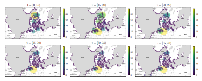Figure 5: Pointmap showing the normalised average supply over time intervals [t − 5,t) in the Baltic Sea region. Best viewed in colour.

Et = {{Et,l = et,l}ml=0,…, {Et,l = et,l}ml=0}, (14) with each element E_t,l originally being directly in E_t and each subset {E_t,l = e_t,l}^m_l=0 concerning the same parfactor partition P_t. SA₄PG proceeds by processing each evidence cluster separately. Evidence of each evidence cluster is processed in a sense such that known inequalities and any uncertainty about inequality is counteracted. This is being done by identifying the dominating observation within each evidence cluster {E_t,l = e_t,l}^m_l=0 and apply that observation to all entities within the respective parfactor partition P_t. The dominating observation max(e_t,l) is the observation that can be observed the most within the evidence cluster. Further, in case any other entities in the corresponding parfactor partition are unobserved, we also apply the dominating observation for those. For each entity for which evidence was inferred or dismissed, the violation counter is increased. In case the violation threshold H for an entity is already reached, evidence is no longer inferred or dismissed, but the entity is relieved from its symmetry cluster, i.e., split off from the parfactor group, and from then on considered individually.

In the following, we evaluate MOP₄SA and SA₄PG as part of a case study from the example shipping domain.

6. MOP₄SA and SA₄PG in Application

Since MOP₄SA consists of multiple steps, namely (a) encoding entity behaviour, (b) similarity counting, and (c) clustering, we evaluate each step separately before analysing the overall fitness in conjunction with SA₄PG, as introduced in Section 5.

6.1. The AIS Dataset

To setup a DPRM as shown in Figure 1a, we use historical vessel movements from 2020 based on automatic identification system (AIS) data^[3] provided by the Danish Maritime Authority for the Baltic Sea. AIS data improves the safety and guidance of vessel traffic by exchanging navigational and other vessel data. It was introduced as a mandatory standard by the International Maritime Organisation (IMO) in 2000. Meanwhile, AIS data is used in many different applications in research, such as trade flow estimation, emission accounting, and vessel performance monitoring [43]. Preprocessing for retrieving variables Supply and Idle for 367 defined Zones can be found on GitHub^[4]. Figure 5 gives an idea on how supply evolves over time t in the Baltic Sea region. Each point illustrates the normalised cargo supply amount in tons. For sake of simplicity, we only plot supply independent of idle times here. We can see, that in the beginning of the year (for 0 < t < 20) the supply in the northern regions, i.e. the need for resources, is higher, while for the rest of the year (for 20 < t < 40) the supply slowly decreases and increases in the southern regions. The important part here is, that the supply for 20 < t < 40 in the respective regions is more or less constant over a longer period of time.

Algorithm 1: Preventing Groundings

Input: DPRM (G₀,G_→), Evidence- E and Querystream Q,

Order d, Delay τ, Symmetry Clusters C for each parfactor g_i ∈ G₀ do

v_|gi ← init violoation map // see Definition 5.1

for t = 0,1,…,T do

E_t ← get evidence from evidence stream E

Rearrange E_t to create evidence clusters according to parfactor partition P_t // see Definition 5.2 for each evidence cluster E_t do max(e_t,l) ← get dominating observation

// Align Evidence

for each observation in E_t,l do if e_t,l , max(e_t,l) and viol(x_i) < H then Dismiss observation e_t,l viol(x_i) ← viol(x_i) + 1

// Infer Evidence for each unobserved entity x_j in P_t do Set E_t,_l(x_j) = max(e_t,_l)

Answer queries Q_t from query stream Q

The idea behind MOP₄SA is to identify periods of time with similar behaviour for multiple entities. That means in our application, identifying zones with similar supply (or more specifically in the multivariate context supply/idle times) over a period of time.

Next, we look into clustering based on the similarity graph as an outcome of similarity counting after applying the symbolisation.

6.2. Multivariate Symbolisation Scheme for Temporal Similarity Clustering

According to the procedure as introduced in Section 4.1.3, we apply the symbolisation scheme on the multivariate supply/idle-time time series as encoded in the parfactor gⁱ_t and create one similarity graph as the basis for clustering. We compare different clustering algorithms as follows. Unfortunately, classical clustering methods do not achieve good results in high-dimensional spaces, like for DPRMs, which are specifically made to represent large domains. Problems that classical clustering approaches have is, that the smallest and largest distances in clustering differ only relatively slightly in a high-dimensional space [44]. For DPRMs, a similarity graph, representing the similarity of entities z ∈ D(Z), contains

fully-connected nodes in the worst case, where Z is a logvar representing a set of entities whose entity pairs share similar behaviour for least one time step. Here, Eq. (15) also corresponds to the number of dimensions a clustering algorithm has to deal with.

6.2.1     An Informal Introduction to Clustering

Generally, clustering algorithms can be divided into the four groups (a) centroid-based clustering, (b) hierarchical clustering, (c) graphbased clustering, and (d) density-based clustering.

We already pointed out the problem that classical clustering algorithms suffer due to their distance measures, which do not work well in high dimensional spaces. Especially centroid-based clustering approaches, like the well-known k-means algorithm or Gaussian Mixture Models, suffer, as they expect to find spherical or ellipsoidal symmetry. More specifically, in centroid-based clustering the assumption is that the points assigned to a cluster are spherical around the cluster centre and therefore no good clusters can be found due to the relatively equal distances. In hierarchical clustering time and space complexity is especially bad since the graph is iteratively split into clusters. Graph-based clustering algorithms, like spectral clustering, is known as being especially robust for high-dimensional data due to performing dimensionality reduction before running clustering [45]. One disadvantage, which also applies to clustering algorithms above, is that the number of clusters need to be specified as a hyperparameter in advance. In contrast, in density-based clustering approaches, like DBSCAN, the number of clusters are determined automatically while also handling noise. DBSCAN is based on a high-density of points. That means, clusters are dense regions, which are identified by running with a sliding window over dense points, making DBSCAN cluster shape independent.

For these reasons, we will compare spectral clustering and DBSCAN as part of MOP₄SA as follows. We start by informally introducing Spectral Clustering and DBSCAN.

DBSCAN works by grouping together points with many nearby neighbours, denoting points lying outside those regions as noise. In DBSCAN the two parameters  and minPoint need to be provided from the outside, which correspond to the terms Density Reachability and Density Connectivity respectively. The idea behind DBSCAN is to identify points, that are reachable from another if it lies within a specific distance from it (Reachability), identifying core, border and noise points as the result of transitively connected points (Connectivity) [46]. More specifically, a core point is a point that has m points within a distance of n from itself, whilst a border point has at least one core point within the distance of n. All other points are considered as noise. The algorithm itself proceeds by randomly picking up a point from the dataset, that means, picking one node from the similarity graph, until every point was visited. All minPoint-points within a radius of  around the randomly chosen point are considered as one cluster. DBSCAN proceeds by recursively repeating the neighbourhood calculations for each neighbouring point, resulting in n clusters.

Spectral Clustering involves dimensionality reduction in advance before using standard clustering methods such as k-means. For dimensionality reduction, the similarity graph W is transformed into the so-called graph Laplacian matrix L, which describes the relations of the nodes and edges of a graph, where the entries are defined by

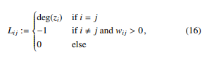with deg(z_i) = ^P|D_j=⁽₁^Z)| w_ij. For decorrelation, data in the graph Laplacian matrix L is decomposed into its sequence of eigenvalues and the corresponding eigenvectors. The eigenvectors form a new uncorrelated orthonormal basis and are thus suitable for standard clustering methods. The observations of the reduced data matrix whose columns contain the smallest k eigenvectors can now be clustered using k-means. An observation assigned to cluster C_i with i = 1,…,k can then be traced back to its entity z ∈ D(Z) by indices. We evaluate both clustering approaches as part of SA₄PG in Section 6.3. To improve comparability, we compare both clustering approaches as described in the next Section.

6.2.2     Clustering Comparison Approach

We compare DBSCAN and Spectral Clustering in MOP₄SA by identifying clusters with each clustering approach and use resulting clusters within SA₄PG respectively, i.e., run SA₄PG once using clusters determined by DBSCAN and once using clusters determined by Spectral Clustering.

Since DBSCAN is able to automatically determine the numbers of clusters, we use DBSCAN to identify same and provide the resulting number of clusters as a parameter when performing Spectral Clustering. As DBSCAN is capable to also classifies noise, i.e., entities, which cannot be assigned to a cluster, we use the number of points classified as noise plus the number of clusters as the number of total clusters in Spectral Clustering. Further, for DBSCAN we provide minPoints = 2 as the minimum number of entities in a cluster to allow for the maximum number of clusters in general. The eps parameter is automatically determined using the kneedle algorithm [47]. For Spectral Clustering we just provide parameter k for the total number of clusters, which was previously determined by DBSCAN. Note that the total number of clusters n, which was determined by DBSCAN, does not necessarily corresponds to the best number of clusters for Spectral Clustering. Nevertheless, we obtain results that show which algorithm, given the same input n, is better at separating entities in the multidimensional space.

In the following, we perform a detailed comparison between the two clustering approaches as part of SA₄PG with different parameters for the symbolisation scheme in MOP₄SA using the approach to compare the two clustering mechanisms as described here.

6.3. Preventing Groundings

MOP₄SA is affected by (a) the efficiency of the clustering algorithm used, (b) the similarity measure itself, (c) and its hyper parameters such as order d, delay τ and δ for the arithmetic mean as defined in Eq. (9). We evaluate MOP₄SA as part of SA₄PG. Specifically, we approximate symmetry clusters using MOP₄SA with different settings and (i) perform inference using the the symmetry clusters to prevent the model from grounding, and (ii) compare it with exact lifted inference and calculate Kullback Leibler divergence (KLD) between query result to determine the error introduced through SA₄PG. A KLD with D_KL = 0 indicates that both distributions are equal. Inference in DPRMs is performed by the lifted dynamic junction tree algorithm. Details can be found in [5].

We ran 54 experiments in total with different parameter combinations d ∈ {2,3,4}, τ ∈ {1,2,3}, δ ∈ {0.05,0.1,0.15} and clustering through Spectral Clustering and DBSCAN. For comparison, we perform query answering given sets of evidence, i.e., we perform inference by answering the prediction query P(Supply_t(Z), Idle_t(Z)) for each time step t ∈ {4,…,51} and obtain a marginal distribution for each entity z ∈ D(Z). We repeat query answering three times, once without preventing any groundings, once with preventing groundings using the clusters determined by DBSCAN, and once again with preventing groundings but using clusters determined by Spectral Clustering for each parameter combinations. Note that we only discuss results for a sub-selection of the parameter combinations, which give good results in terms of accuracy in inference under preventing groundings, while Table 1 and Table 2 at the end of this paper show the full results for all parameter combinations. Table 1 and Table 2 show results for time intervals t ∈ {[5,10),[10,15), [15,20),[20,25),[25,30),[30,35),[35,40),[40,45),[45,50)}.

We evaluate runtime in seconds s, the number of groundings #_gr and KLD D_KL. Note that, #_gr shows the number of clusters after time t, while n shows the initial number of clusters. Thus, the number of additional groundings at a specific timestep equals to #_gr minus n. Preventing groundings aims at keeping a lifted model as long as possible. A basic prerequisite for this is that similarities exists in the data. As to that, the variable n_≥1 shows the number of initial clusters, which contain more than one entity directly after clustering, i.e., clusters in which similarly behaving entities have been arranged. Note that similar to n, n_≥1 does not change over time. With increasing order d the number of neighbouring data points are increasing, i.e., the classification contains more long term patterns. With increasing delay τ, long-term behaviour is extended even further, while also allowing for temporary deviations. For data range dependence, in similarity counting we test different delta δ_≤.

The number of clusters with more than one entity n_>1 relative to the total number of clusters n are important in evaluating how well symmetries are exploited. When n is small, i.e. when n is significantly smaller than the total number of entities |D(Z)|, a value of n_>1 close to n is desirable since it indicates that many entities show symmetries with each other. If n_>1 is significantly smaller than n, then only a few entities show symmetries, which on the one hand leads to a better accuracy in the inference since many entities are considered at a ground level, but on the other hand runtime will suffer greatly. As to that, Figure 6 shows a comparison for different parameter combinations and clustering approaches. The red line denotes the total number of clusters n independently of the number of entities included in a cluster, while the bars only show the number of clusters with more than one entity n_>1. Note that we also include entities, which are treated on a ground level already by the time after learning clusters, in the total number of cluster, i.e., clusters can also only include one entity. Since lifting highly depends on the degree of similarities, only those clusters with more than one entity are of interest. Each pair of bar plots correspond to a different experiment with different parameter combinations.

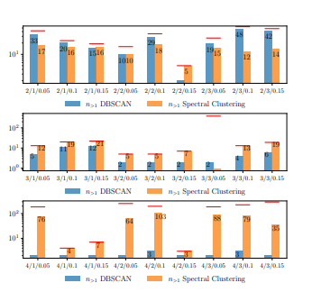Figure 6: Comparison of number of clusters with more than one entity between DBSCAN and Spectral Clustering.

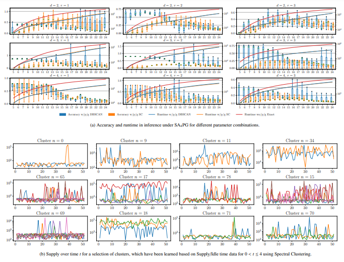Figure 7: Accuracy and runtime data based on query results under SA₄PG including raw supply data for entities within clusters.

Due to space limitations we shorten order d, delay τ and delta δ_leq in the graph by the triple d/τ/δ_leq. From Fig. 6 it is most noticeable that the number of clusters with more than one entity n_≥1 for higher orders d is much less than for lower orders. This intuitively makes sense, since with higher orders d long term behaviour is captured much better than with lower orders and thus only a few clusters can be determined. For d = 2 much more clusters are identified since a smaller time span is considered resulting in a higher possibility of showing similarities. This observation also applies to increasing delays τ. The experiment with order d = 3, delay τ = 3 and delta δ_≤ = 0.05 is a good example for cases where not many similarities have been identified, but many entities are treated on a ground level, i.e., accuracy will be good, but runtime will suffer. In the following, we look at accuracy results and will also come back to this example.

By comparing the KLD D_KL as a result of inference without preventing groundings and with preventing groundings based on clusters determined by DBSCAN and Spectral Clustering, it is noticeable that for clusters determined by Spectral Clustering in average a lower D_KL compared to DBSCAN results. This is explainable with better handling of higher dimensional data in Spectral Clustering. Figure 7a shows a comparison between the accuracy for both cases and different parameter combination. Each subplot corresponds to a different order d and delay τ, while the box-plot itself shows the variation of the accuracy over different deltas δ_≤ = {0.05,0.1,0.15} over time t. Note that we only plot data until t = 24 for better visibility and as the effect of any wrong evidence, which was brought in by preventing groundings, starts to level off. This happens since groundings are only prevented until the threshold H is reached, i.e., any other evidence afterwards at a later timestep balance out the effect of any wrong evidence at an early timestep after learning symmetry clusters. The blue box-plots in Fig. 7a correspond to the KLD D_KL with DBSCAN as the clustering approach in MOP₄SA, while the orange box-plots correspond to the KLD D_KL with on Spectral Clustering as the clustering approach in MOP₄SA. The solid blue, orange and red line correspond to the runtime for answering a query for the specific time step. From the plots, we can see that for higher orders and delays, i.e., with increasing time spans each ordinal represents, that D_KL is decreasing. Considering the total number of clusters for each experiment (see Fig. 6), this follows as not many similarities can be found in the data, but more entities are handled on a ground level, i.e., increasing accuracy. On the other hand, runtime drastically increases as symmetries are no longer exploited. Compared to exact reasoning, runtime is noticeably smaller in inference under SA₄PG. To lock again at the experiment with order d = 3, delay τ = 3 (as highlighted above), the KLD D_KL is considerably small especially for Spectral clustering, but the runtime of the inference is very poor compared to all other experiments.

In SA₄PG, the violation threshold H is set to 5, i.e., groundings due to any inequalities are prevented for an entity H times. After t = 10 the number of groundings #_gr (see Table 1) are still the same as after learning the entity similarity cluster, i.e., all groundings are prevented. It is expected that the majority of groundings are prevented in the initial timesteps after learning the clusters. Still, if entities behave similarity in early timesteps, the threshold H is reached far later in time. Thus, if in clustering based on the similarity graph the entities with similarities are identified better, then groundings will occur much later in time. The longer D_KL stays small, the better cluster fit, i.e, the error introduced in inference through preventing groundings is kept small. In Fig. 7a we see that the accuracy suffers approximately for all experiments around t = 10, i.e, after 4 more timesteps after learning the clusters. Figure 7b depicts raw supply data for a selection of clusters as a result of running MOP₄SA based on data for t = [0,4) with parameters d = 2, τ = 1 and δ = 0.05 for symbolisation and Spectral Clustering. Even though only providing a small amount of training data, we can see that symmetrical behaviour continues for most of the clusters until approx. t = 10, like especially for clusters n ∈ {0,11,34,65,78,69,71} and therefore support the insight, which we have got based on Fig. 7a. For simplicity only raw supply data is plotted even though symmetry clusters are determined based on supply/idle data.

The best results are achieved with Spectral Clustering as part of SA₄PG for the parameter combinations d = 2, τ = 1, δ_≤ = 0.1, d = 3, τ = 3, δ_≤ = 0.1 and d = 3, τ = 2, δ_≤ = 0.05, which we will also further refer to in the following Section. Generally, when reasoning under time constraints, preventing grounds is a reasonable approach as it prevents groundings in the long term and therefore speeds up inference.

Entity similarity can change over time, i.e., to further prevent the model from grounding it is beneficial to relearn symmetry structures at some time. In the following we propose MOP₄SCD and use it to identify points in time when relearning clusters is beneficial.

7. Multivariate Ordinal Pattern for Symmetry Change Detection (MOP₄SCD)

Symmetries in temporal models can change over time as already seen in Fig. 5. Therefore, symmetry cluster, after they have been learned, may only stay valid for a certain period of time. Further, some are valid for a longer period of time, some not. To identify points in time when relearning symmetry clusters is reasonable, we use the similarity graph as an intermediate output of running MOP₄SA and check if the similarity graph has changed significantly. More specifically, we continue running MOP₄SA for every timestep, but instead of for continuously relearning symmetry clusters, we prevent relearning clusters in MOP₄SA after the initial sync run until the graph has changed significantly enough. To identify such points in time with a significant change, we introduce MOP₄SCD taking as inputs a similarity graph for two consecutive timesteps and calculating a distance measure between both. In case the distance measure is above a certain threshold we consider those points as change points to trigger the cluster relearning process. MOP₄SCD is based on the assumption, that clusters no longer stay valid, if entities within a cluster no longer show the same similarity to its cluster entities as in the previous timesteps, i.e., the similarity counts is no longer proportionally scaling as before. Those entities might transition to another cluster, since its showing more similarity with another cluster. Informally, if the similarity graph changes over time in a constant and balanced way, symmetry clusters stay valid, but if the similarity graph changes over time in an unbalanced manner, i.e., if similarity counts change significantly, there is a change in the structure of the symmetry clusters. To illustrate that, let us look at Figure 8. The Figure shows a similarity graph based on which two clusters have been identified.

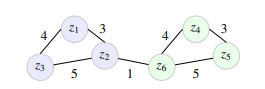Figure 8: Overview of potential unbalanced changes in a similarity graph.

Nodes S ¹ = {z₁,z₂,z₃} (coloured in blue) denote a cluster S ¹ and the nodes S ² = {z₄,z₅,z₆} (coloured in green) denote another cluster S ². Both clusters are connected through nodes z₂ and z₆ since for both a similarity was measured at any timestep before learning clusters. Relearning clusters becomes necessary if the cluster structure itself changes. This happens either

• if similarities between entities of different clusters changes,

e.g., if the similarity between z₂ and z₆ increases and might require to merge the clusters or even split them into more than two clusters, which we denote as a unbalanced interclusteral change,

• or if similarities within a cluster change disproportionately, e.g., if similarities for S ² changes only for a subset of the entities such as for z₄ and z₅ but not proportionally for all entities such as z₄ and z₆ and z₆ and z₅ requiring to split the cluster even further, which we denote as a unbalanced intraclusteral change.

As follows we define both unbalanced interclusteral and intraclusteral change measures and combine both into a distance measure denoting the unbalanced change between consecutive timesteps. Both unbalanced inter- and intraclusteral changes are determined based on the similarity graph W^t from the current to the next time step W^t+1 under current symmetry clusters S, with interclusteral changes defined as

where [x] = 1 if x and, 0. Both d_inter and d_intra are merged into one combined measure with

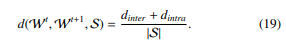Simply speaking, d_inter counts the number of increases in weights across different clusters S ⁱ and S ^j such as shown in Fig. 8 for entities z₂ and z₆. The resulting count is normalised by dividing through the number of comparison between entity pairs of the clusters en(S ⁱ) and en(S ^j), resulting in measure between 0 and 1 with a value close to 1 denoting a maximum dissimilarity. Similarly, d_intra counts the occurrences of no weight increases within entity pairs of a similar cluster S ⁱ. To ensure that entities within a cluster continue to behave the same, weights should proportionally increase equally distributed within the cluster. If there is no increase in weights most likely the entities discontinue to behave similarly. The resulting count is equally normalised with a value close to 1 denoting a maximum dissimilarity. Finally, both d_inter and d_intra are combined in a single measure also count normalised to determine a distance measure between 0 and 1. If d(W^t, W^t+1, S) = 0, the change in the similarity graph is balanced, if d(W^t, W^t+1, S) > 0, it is unbalanced. If d(W^t, W^t+1, S) > b, b ∈ N_>0 it may be worthwhile to (re)perform clustering and (re)build symmetry clusters.

As follows, we evaluate MOP₄SCD based on clusters determined by MOP₄SA for the same parameters as in the experiments performed in Section 6.

8.  MOP₄SCD in Application

We evaluate MOP₄SCD based on clusters determined using

MOP₄SA as described in Section 6. Since Spectral Clustering works better than DBSCAN in identifying clusters, we here only use clusters determined by Spectral Clustering as part of MOP₄SA. We run experiments 27 experiments in total for the same parameter combinations d ∈ {2,3,4}, τ ∈ {1,2,3} and δ ∈ {0.05,0.1,0.15} as in Section 6. For each experiment we calculate d(W^t, W^t+1, S) for timesteps t = 5,…,51. Clusters are learned based on a similarity graph with data for t = 1,…4.

In this Section we discuss results for a sub-selection of the parameter combinations, which give good results in terms of accuracy in inference under preventing groundings as seen in Section 4, while Table 3 at the end of this paper shows detailed results for all parameter combinations. Each column in Table 3 shows the distance measure for consecutive timesteps, e.g., for t = 5, the distance is derived based on the similarity graph for timestep t = 4 to t = 5, i.e., d(W⁴, W⁵, S). Note that since d(W⁴, W⁵, S) is calculated for two consecutive timesteps, the distance measure has to be added up over time to derive the overall distance between more then two timesteps. Overall, the distance measure varies for different parameter combinations with in the optimal case showing an unbalanced change in weights of approximately 1.6% and in the worst case of approximately 22.4% between two consecutive timesteps. The distance measure is highly affected by the number of clusters n. In the case that the number of clusters with more than one entity n_>1 is considerably small compared to the total number of clusters n, the distance measure d(W^t, W^t+1, S) is also considerably low since d_inter and d_intra, see Eq. (17) and Eq. (18), always return no unbalanced change for clusters with just one entity, i.e., for entities which are already being treated on a ground level. MOP₄SA aims at preventing groundings to speed up inference, i.e., lead to an increase in runtime. Therefore, choosing parameters d, τ and δ for MOP₄SA and consequently for MOP₄SCD is a trade-of between losses in accuracy and a speed up in inference.

The parameter combinations d = 2, τ = 1, δ_≤ = 0.1, d = 3, τ = 3, δ_≤ = 0.1 and d = 3, τ = 2, δ_≤ = 0.05 give good results in MOP₄SA as shown in Section 6. Results for MOP₄SCD also support this. Figure 9 shows the KLD D_KL in conjunction with results from MOP₄SCD. Each subplot corresponds to a different parameter combination with the blue line corresponding to the KLD D_KL, the solid red line to the distance measure d(W^t, W^t+1, S) for two consecutive timesteps t and t + 1 and the dashed red line for the cumulative distance measure, i.e., from t = 0 until the current timestep t. Note that the cumulative distance is log scaled and can be read of from the right y-axis. The highlighted red area in each subplots mark the interval when the cumulative distance measure becomes greater then 50% until it has reached 100%, i.e., with a change of 100% that all relations between all entities have been affected.

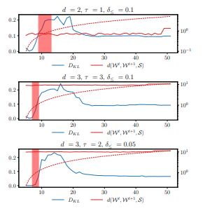Figure 9: Results of MOP₄SCD for three parameter combinations which show the best results for MOP₄SA and SA₄PG. Further results can be found in the appendix.

Similar to the experiments in Section 6, clusters S have been determined by MOP₄SA based on data for 0 > t ≤ 4. For all upcoming timesteps the clusters S have been used to prevent groundings, i.e., execute SA₄PG as part of inference, see Algorithm 1. The KLD D_KL for all experiments as shown in Fig. 9 similarly raises up to a value of approx. 0.25 with its peak around t = 15. In contrast d(W^t, W^t+1, S) varies across experiments and has for the experiment with parameter combination d = 2, τ = 1 and δ_≤0.1 its best value of approx. 0.1, i.e, a unbalanced change of approx. 10% over time. For the two other experiments d(W^t, W^t+1, S) is with 0.22 similar. Correspondingly, the cumulative distance reaches a value of 0.5 at timestep t = 9 until it reaches a value of 1 at t = 14 for the first experiment, while for the two other experiments the cumulative distance reaches a value of 0.5 at t = 7 and a value of 1 already at t = 9. I.e., clusters S are valid for a longer period of time using MOP₄SA with a parameter combination of d = 2, τ = 1, δ_≤ = 0.1. Further, for that parameter combination, D_KL settles off once a cumulative distance of 1 has reached. Settling off happens due to the amount of new evidence leading to more groundings removing the effect of any wrongly introduced evidence in previous timesteps. Relearning clusters at a threshold of 0.5 is here beneficial to prevent the D_KL from further increasing. That means relearning at t = 9, i.e., clusters are valid for approx. 4 timesteps after learning them, which corresponds to a full month in our example application and therefore is a good result to considerably speed up inference while only introducing a small error in inference.

9. Conclusion and Future Work

Evidence lead to groundings in dynamic probabilistic relational models over time, negating runtime benefits in lifted inference. This paper provides MOP₄SA, SA₄PG and MOP₄SCD as a rich toolset to identify model symmetries as part of the model construction process, use those symmetries to maintain a lifted representation by preventing groundings a priori and detect changes in model symmetries after the model construction process. Preventing groundings a priori to maintain any lifted representation is important in lifted inference to preserve its runtime benefits. MOP₄SA detects symmetries across entities of the models domain using a multivariate ordinal pattern symbolisation approach and building a similarity graph for spectral clustering to identify sets of entities with symmetrical behaviour regarding a context of the model (symmetry clusters). Symmetry clusters are used in SA₄PG as part of query answering to prevent any unnecessary model splits by evidence, e.g., due to one time events. Symmetry structures can change over time, which MOP₄SCD detects based on the similarity graph, an intermediate output of MOP₄SA, and provide a distance measure denoting the degree of any unbalanced structural change to identify points in time when relearning symmetry clusters is beneficial.

The main contribution of this paper are the extension by theoretical and experimental results on the original papers [1, 2] and the introduction of MOP₄SCD as a mechanism to detect structural changes to complement MOP₄SA, SA₄PG as a rich toolset to prevent groundings a priori. We show, that MOP₄SA requires only a small amount of training data to come up with a good approximation of symmetry structures. Generally, MOP₄SA aims at determining symmetry structures which stay valid for shorter time periods. This follows, since MOP₄SA is not capable to capture any reoccurring patterns or periodicity, e.g., due to seasonality. MOP₄SA can be extended to capture such behaviour, but this would also increase the complexity of the overall approach. Due to this and since capturing symmetries for longer time spans, especially in real-world applications which normally change much faster, is not feasible, we focus with MOP₄SA as being a simple and easy to compute framework, requiring only few historical data points for learning, to identify symmetries for the short term future. In addition to MOP₄SA, MOP₄SCD supports in inference by identifying points in time when relearning clustering for SA₄PG is reasonable.

With preventing groundings a priori we complement existing approaches, which focus on retaining lifted representation after a model has already been splitted. In general, our approach works well with any other approach undoing splits after they occurred when moving forward in time, e.g., in message passing by merging sets of entities when those align again, denoted as temporal approximate merging, as proposed in [25]. Combining both kind of approaches brings together the best of both worlds: (a) While with determining approximate model symmetries a priori, we can use the full amount of historical training data to prevent groundings, (b) and with temporal approximate merging, we can merge non-preventable parfactor splits even after they occurred, i.e., a posterior.

Since MOP₄SA is designed to work with small amounts of data to provide symmetry clusters very quickly for the short term future, the overhead MOP₄SA and MOP₄SCD bring into query answering need to be kept to a minimum. Applying the symbolisation scheme to identify symmetries is already a suitable mechanism, but with the clustering approach we still depend on existing approaches, which are considerably costly. The investigation of more performant clustering approaches, e.g., taking advantage of some sort of incremental changes to clustering after the initial learning step, are left for future work.

List of Symbols

R	set of random variables
L	set of logical variables
Φ	set of factor names
D	set of entities
D(L)	domain of a logvar
C,(X,CX)	constraint restricting logical variables
A(L1,…, Ln)	parameterised logical variable (PRV)
g,φ(A)|C	parfactor
gr(P)	grounding
lv(P)	logical variables
R(A)	range of a PRV
G	model
Gt	local model
E	evidence, set of events
Q	query term
X	multivariate time series
τ	delay between successive time points
d	order of ordinal pattern
wij	similarity count
W	similarity graph
S	symmetry cluster
en(S)	objects in a symmetry cluster
S	set of symmetry clusters
P	parfactor partition
L	Laplacian matrix
DKL	Kullback-Leibler divergence
δ≤	mean delta
d(Wt, Wt+1, S) similarity change measure

 

1. N. Finke, M. Mohr, “A Priori Approximation of Symmetries in Dynamic Probabilistic Relational Models,” in S. Edelkamp, R. Mo¨ ller, E. Rueckert, editors, KI 2021: Advances in Artificial Intelligence, 309–323, Springer International Publishing, Cham, 2021.
2. N. Finke, R. Mo¨ ller, M. Mohr, “Multivariate Ordinal Patterns for Symmetry Approximation in Dynamic Probabilistic Relational Models,” in AI 2021: Ad- vances in Artificial Intelligence – 34rd Australasian Joint Conference, Lecture Notes in Computer Science (LNCS), Springer International Publishing, In Press.
3. N. Finke, M. Gehrke, T. Braun, T. Potten, R. Mo¨ller, “Investigating Matureness of Probabilistic Graphical Models for Dry-Bulk Shipping,” in M. Jaeger, T. D. Nielsen, editors, Proceedings of the 10th International Conference on Proba- bilistic Graphical Models, volume 138 of Proceedings of Machine Learning Research, 197–208, PMLR, 2020.
4. Y. Xiang, K.-L. Poh, “Time-Critical Dynamic Decision Making,” 2013.
5. M. Gehrke, T. Braun, R. Mo¨ller, “Lifted Dynamic Junction Tree Algorithm,” in Proceedings of the International Conference on Conceptual Structures, 55–69, Springer, 2018.
6. D. Poole, “First-order Probabilistic Inference,” in Proc. of the 18th International Joint Conference on Artificial Intelligence, 985–991, 2003.
7. D. Akyar, “The Effects of Global Economic Growth on Dry Bulk Shipping Markets and Freight Rates,” 2018.
8. Z. Wang, X. Wu, K. L. Lo, J. J. Mi, “Assessing the management effi- ciency of shipping company from a congestion perspective: A case study of Hapag-Lloyd,” Ocean & Coastal Management, 209, 105617, 2021, doi: https://doi.org/10.1016/j.ocecoaman.2021.105617.
9. C. Jiang, Y. Wan, A. Zhang, “Internalization of port congestion: strategic effect behind shipping line delays and implications for terminal charges and investment,” Maritime Policy & Management, 44(1), 112–130, 2017, doi: 10.1080/03088839.2016.1237783.
10. T. Notteboom, “The Time Factor in Liner Shipping Services,” Maritime Eco- nomics and Logistics, 8, 19–39, 2006, doi:10.1057/palgrave.mel.9100148.
11. M. Niepert, G. Van den Broeck, “Tractability through Exchangeability: A New Perspective on Efficient Probabilistic Inference,” in AAAI-14 Proceedings of the 28th AAAI Conference on Artificial Intelligence, 2467–2475, AAAI Press, 2014.
12. G. V. den Broeck, M. Niepert, “Lifted Probabilistic Inference for Asymmetric Graphical Models,” CoRR, abs/1412.0315, 2014.
13. N. Taghipour, D. Fierens, J. Davis, H. Blockeel, “Lifted Variable Elimination: Decoupling the Operators from the Constraint Language,” Journal of Artificial Intelligence Research, 47(1), 393–439, 2013.
14. K. Kersting, “Lifted Probabilistic Inference,” in Proceedings of the 20th Euro- pean Conference on Artificial Intelligence, ECAI’12, 33–38, IOS Press, NLD, 2012.
15. G. Van den Broeck, A. Darwiche, “On the Complexity and Approximation of Binary Evidence in Lifted Inference,” in C. J. C. Burges, L. Bottou, M. Welling,
    Z. Ghahramani, K. Q. Weinberger, editors, Advances in Neural Information Processing Systems, volume 26, Curran Associates, Inc., 2013.
16. P. Singla, A. Nath, P. Domingos, “Approximate Lifting Techniques for Be- lief Propagation,” in Proceedings of the Twenty-Eighth AAAI Conference on Artificial Intelligence, AAAI’14, 2497–2504, AAAI Press, 2014.
17. P. Singla, P. Domingos, “Lifted First-Order Belief Propagation,” in Proceed- ings of the 23rd National Conference on Artificial Intelligence – Volume 2, AAAI’08, 1094–1099, AAAI Press, 2008.
18. B. Ahmadi, K. Kersting, M. Mladenov, S. Natarajan, “Exploiting symmetries for scaling loopy belief propagation and relational training,” Machine Learning, 92, 91–132, 2013.
19. C. Sutton, A. Mccallum, “Piecewise Training for Structured Prediction,” Ma- chine Learning, 77, 165–194, 2009, doi:10.1007/s10994-009-5112-z.
20. D. Venugopal, V. Gogate, “Evidence-Based Clustering for Scalable Inference in Markov Logic,” in T. Calders, F. Esposito, E. Hu¨llermeier, R. Meo, editors, Machine Learning and Knowledge Discovery in Databases, 258–273, Springer Berlin Heidelberg, Berlin, Heidelberg, 2014.
21. P. Miettinen, T. Mielika¨inen, A. Gionis, G. Das, H. Mannila, “The Discrete Basis Problem,” in J. Fu¨rnkranz, T. Scheffer, M. Spiliopoulou, editors, Knowl- edge Discovery in Databases: PKDD 2006, Springer Berlin Heidelberg, Berlin, Heidelberg, 2006.
22. N. Metropolis, A. W. Rosenbluth, M. N. Rosenbluth, A. H. Teller, E. Teller, “Equation of State Calculations by Fast Computing Machines,” The Journal of Chemical Physics, 21(6), 1087–1092, 1953.
23. W. K. Hastings, “Monte Carlo Sampling Methods Using Markov Chains and Their Applications,” Biometrika, 57(1), 97–109, 1970.
24. A. Nath, P. Domingos, “Efficient Lifting for Online Probabilistic Inference,” volume 2, 2010.
25. M. Gehrke, R. Mo¨ ller, T. Braun, “Taming Reasoning in Temporal Probabilis- tic Relational Models,” in Proceedings of the 24th European Conference on Artificial Intelligence (ECAI 2020), 2020, doi:10.3233/FAIA200395.
26. R. Agrawal, C. Faloutsos, A. Swami, “Efficient similarity search in sequence databases,” in Lecture Notes in Computer Science, volume 730, Springer Verlag, 1993.
27. E. Keogh, K. Chakrabarti, M. Pazzani, S. Mehrotra, “Dimensionality Reduc- tion for Fast Similarity Search in Large Time Series Databases,” in Knowledge and Information Systems, 263–286, 2001, doi:10.1021/acsami.7b03579.
28. S. Kramer, “A Brief History of Learning Symbolic Higher-Level Represen- tations from Data (And a Curious Look Forward),” in Proceedings of the Twenty-Ninth International Joint Conference on Artificial Intelligence, IJCAI- 20, 4868–4876, 2020.
29.  J. B. Kruskal, M. Liberman, “The Symmetric Time Warping Problem: From Continuous to Discrete,” in Time Warps, String Edits and Macromolecules: The Theory and Practice of Sequence Comparison, Addison-Wesley Publishing Co., 1983.
30. C.-C. M. Yeh, Y. Zhu, L. Ulanova, N. Begum, Y. Ding, H. A. Dau, D. F. Silva, Mueen, E. Keogh, “Matrix Profile I: All Pairs Similarity Joins for Time Series: A Unifying View That Includes Motifs, Discords and Shapelets,” in 2016 IEEE 16th International Conference on Data Mining (ICDM), 1317–1322, 2016.
31. F. Petitjean, J. Inglada, P. Gancarski, “Satellite Image Time Series Analysis Under Time Warping,” IEEE Transactions on Geoscience and Remote Sensing, 50(8), 2012.
32. S. Salvador, P. Chan, “FastDTW: Toward Accurate Dynamic Time Warping in Linear Time and Space,” 70–80, 2004.
33. D. F. Silva, G. E. A. P. A. Batista, “Speeding Up All-Pairwise Dynamic Time Warping Matrix Calculation,” in Proceedings of the 2016 SIAM International Conference on Data Mining, 837–845, Society for Industrial and Applied Mathematics, 2016.
34. B. Chiu, E. Keogh, S. Lonardi, “Probabilistic Discovery of Time Series Mo- tifs,” in Proceedings of the Ninth ACM SIGKDD International Conference on Knowledge Discovery and Data Mining, 493–498, 2003.
35. C. Bandt, B. Pompe, “Permutation Entropy: A Natural Complexity Measure for Time Series,” Physical Review Letters, 88(17), 4, 2002.
36. M. Mohr, F. Wilhelm, M. Hartwig, R. Mo¨ ller, K. Keller, “New Approaches in Ordinal Pattern Representations for Multivariate Time Series,” in Proceed- ings of the 33rd International Florida Artificial Intelligence Research Society Conference, 2020.
37. K. Keller, T. Mangold, I. Stolz, J. Werner, “Permutation Entropy: New Ideas and Challenges,” Entropy, 19(3), 2017.
38. A. B. Piek, I. Stolz, K. Keller, “Algorithmics, Possibilities and Limits of Ordinal opies,” Entropy, 21(6), 2019.
39. K. Keller, S. Maksymenko, I. Stolz, “Entropy Determination Based on the Or- dinal Structure of a Dynamical System,” Discrete and Continuous Dynamical Systems – Series B, 20(10), 3507–3524, 2015.
40. I. Stolz, K. Keller, “A General Symbolic Approach to Kolmogorov-Sinai En- tropy,” Entropy, 19(12), 2017.
41. A. Antoniouk, K. Keller, S. Maksymenko, “Kolmogorov-Sinai entropy via separation properties of order-generated σ-algebras,” Discrete & Continuous Dynamical Systems, 34(5), 1793–1809, 2014.
42. K. Keller, “Permutations and the Kolmogorov-Sinai Entropy,” Discrete & Continuous Dynamical Systems, 32(3), 891–900, 2012.
43. D. Yang, L. Wu, S. Wang, H. Jia, K. X. Li, “How big data enriches maritime research – a critical review of Automatic Identification System (AIS) data applications,” Transport Reviews, 39(6), 755–773, 2019, doi: 10.1080/01441647.2019.1649315.
44. R. Bellman, Adaptive control processes: A guided tour, Princeton legacy library, Princeton University Press, 2015.
45. A. L. Bertozzi, E. Merkurjev, “Chapter 12 – Graph-based optimization ap- proaches for machine learning, uncertainty quantification and networks,” in
    R. Kimmel, X.-C. Tai, editors, Processing, Analyzing and Learning of Images, Shapes, and Forms: Part 2, volume 20 of Handbook of Numerical Analysis, 503–531, Elsevier, 2019.
46. E. Schubert, J. Sander, M. Ester, H. P. Kriegel, X. Xu, “DBSCAN Revisited, Revisited: Why and How You Should (Still) Use DBSCAN,” ACM Trans. Database Syst., 42(3), 2017, doi:10.1145/3068335.
47. V. Satopaa, J. Albrecht, D. Irwin, B. Raghavan, “Finding a ”Kneedle” in a Haystack: Detecting Knee Points in System Behavior,” in 2011 31st Interna- tional Conference on Distributed Computing Systems Workshops, 166–171, 2011, doi:10.1109/ICDCSW.2011.20.

(Click Here)