1. Introduction

In a manufacturing system, scheduling jobs on a single machine consists of sequencing them through a dispatch rule; that establishes the order of processing based on parameters such as the delivery date, the order of arrival or the processing time. In this sense, the objective of job scheduling is the performance optimization metric in terms of time or cost [1-3].

On the other hand, agile manufacturing refers to the production approach to re-spond quickly to uncertain aspects such as process technologies, customer demand or changing requirements; to achieve this, flexible manufacturing systems are used. In these systems, operations sequences and dispatch strategies are very important to respond in an agile manner [4]. In the present work, the process times are studied as stochastic variables, since this has significant effects in the flexible manufacturing system [5], allowing to measure how robust the solution is when processing times are used according to a certain probability distribution. Such measures can prevent wrong decisions [6]; although these times may vary due to clients requiring certain specifications and tasks can be done by a human or a robot. Additionally, diverse customer requirements make it difficult to accurately estimate processing times.

Agile manufacturing requires managing change with flexibility while main-taining high service levels, just-in-time deliveries, and low production costs [6,7]. Given the above, for a manufacturing company that produces under an agile approach, it will be of interest to know the sensitivity of the total cost of each sequencing rule with respect to variations in the unit costs of maintaining inventory and penalties for late deliveries. The goal of analyzing such sensitivity is to control and ensure the agility of the production system in a changing environment. In this sense, knowing the sensi-tivity of the total cost for each sequencing rule would allow, for example, to determine improvement objectives in the inventory and material handling system to maintain early production at a lower cost. Also, the sensitivity analysis would lead to establish negotiation strategies with customers on penalty policies for late production and select the sequencing rule that minimizes the two above costs and, at the same time, provides greater robustness in an environment that makes these costs vary.

For this reason, the motivation of this article is to present a sensitivity analysis that will serve as an instrument to support decision-making in the selection of sequencing rules. Particularly, when the costs of early and late production vary due to a changing environment, it is important to select the priority rule that is the more robust. Changing the processing times is motivated by the fact that the sequencing problems not only have a combinatorial structure, but also a temporal structure [8]. More specifically, changing the processing time of activities will also change the completion time of the jobs later, changing its delivery date, the parameters used to decide the optimal se-quence (such as the average number of late jobs) and, therefore, the optimal sequence. Sensitivity analysis in this area is important because we live in an environment where processing times can change [9,10], as in agile manufacturing.

The article is structured as follows. In section 2, a brief analysis of the state of the art on agile manufacturing, stochastic dispatch rules, and their sensitivity analysis is carried out. In section 3, the problem and the method used to simulate production runs with stochastic processing times are described. In section 4, the simulation results are presented, analyzing the sensitivity of the total cost per sequencing rule in two steps: first, three cases of the Holding Cost – Penalty Cost relationship (greater than, less than and equal to) are identified and how they impact the total cost. Once it is observed whether the cases are significant for the selection of sequencing rules, one of the two costs is varied while the other remains fixed to observed how the total cost changes. Finally, in section 5, the results obtained and their applicability in companies that produce under an agile approach are discussed.

2. Literature review

Since 1990, research has been done on sensitivity problems of sequencing prob-lems, for example, in[11-13]. The precedence of operations has been studied in [14] and [15], the sensitivity of sequencing problems in parallel machines has also been experimented in [16].  In [17] the researchers examine single machine problems considering time intervals and discrete processing times, [18] and [19] also analyze similar cases. Cost sensitivity is important because costs are not always adequately estimated or vary due to changing customers’ requirements. Thus, it must be resolved what would happen if these costs change [20].

There are works that present the choice for accepting or rejecting a job according to its penalty depending on its cost. For example, in [21]  the researchers use a single machine with stochastic processing times. In [22] test priority rules with stochastic process times are used, but without considering cost. These authors show that the priority rules in a single machine with stochastic processing times are of current interest, because the single machine models have properties that more complex models have [4]. For example, a more complicated system that have a bottleneck is similar to a single machine model. Agile manufacturing deals with high human mix between humans and robots in collaborative manufacturing facilities, which creates uncertainty in job processing times [23-25]. Therefore, it is necessary to respond quickly to unforeseen customer demands. In this kind of manufacturing systems there is also a need of active and proactive schedules [26], in which the decision maker thinks (or rethinks) in how the activities need to be prioritized to be ready for any possible scenario [27]. This high variation of production requirements makes it challenging to find the optimal solution at the lowest cost [28], or to find the most robust solution. For this, in [23] is proposed a sequencing and dispatch method for facilities where humans and robots are mixed, while handling uncertainty in process times to minimize the variability of the solution. In [28] the authors optimize the production line that works with parallel machines that work at different speeds, whereas in [29] propose an adaptive sequencing and dispatch method for human-robot collaborative manufacturing sys-tems where policy is dynamically adjusted using petri nets.

In [30] they suggest a mathematical model for the sequencing problem in a mixed model with high variety. To achieve this, the authors developed a heuristic solution to minimize the variability of the workload. In [27] performed a robust programming in the automatic supply chain presenting a hybrid store flow with job shop type processes, where multiple objectives are handled in the presence of capacity changes. In [31], they performed an optimization through simulation that allows dealing with the programming of vehicles and machines in a flexible system with stochastic elements included. Furthermore, a genetic algorithm is used to reduce the number of replicas. In [32] the authors worked with an assembly line where multiple products were manufactured with different demand, delivery dates and the variation in the material, to minimize the makespan and the cost of penalty for late delivery. Table 1 presents a comparison of these works and the proposal.

Table 1: Comparison of the relevant aspects of articles that address the Sequencing Problem in Agile. Own elaboration

Work	Uncertainty and robustness	Multiple machines	Use simulation	Optimized objective	Costs sensitivity
[23]	yes	yes	yes	Variability in the solution	no
[28]	no	yes	yes	Multiobjective (production and energy)	no
[29]	yes	no	no	Idle time	no
[30]	no	yes	no	Workload	no
[27]	yes	yes	no	Makespan	no
[31]	yes	yes	yes	Multiobjective (makespan, tardiness)	no
[32]	yes	yes	no	Multiobjective (variation in material, makespan, penalty cost)	no
Proposal	yes	no	yes	Total cost, total early and late production time	yes

These works present different methodologies for agile manufacturing. What is different about the proposal in this article is the cost sensitivity analysis, since the total cost as a performance metric allows to control and ensure an agile manufacturing system in a changing environment in a viable way. Additionally, to check the robustness of the solution in the dispatch rules, stochastic processing times with a normal distribution are used through the inverse transform method[1] that is explained in [33]. The normal distribution for the processing times is used because the convolution property that it has, and the sum of the processing times is needed as it will be explained later, and, last but not least, each of these times has a normal distribution. Given two normal probability density functions and , it is proved in the literature [34] that the convolution of these two functions is a normal probability distribution function with mean and variance. This article presents jobs that need to go through a manufacturing robot with different processing times, but sometimes need to be processed by humans to meet customers’ requirements. The method to perform the sensitivity analysis is presented in section 3.

The research questions are the following:

RQ1. If lead times are stochastic, what is the priority rule for assigning jobs that should be chosen to minimize costs?

RQ2. If processing times are stochastic, what is the most robust priority rule, that is, with less variability in terms of costs?

3. Method

3.1.  Problem description

Let be a problem of one robot ( with jobs to be processed. Additionally,

 stochastic processing time of the job  in an arbitrary distribution.

 the due date of the job  represents the shipping or completion date, and the completion of a job after a due date is allowed with a certain penalty.

 time in which the job  is completedthe completion of the last job or makespan

To make the decisions, the priority rules listed below are used.

 = Shortest processing time, jobs are sorted according to processing times in ascending order.

 = Longest processing time, jobs are sorted according to processing times in descending order.

 = Earliest due date, the jobs enter the sequence according to the earliest due date and finish on the latest.

 = First Coming First Served, the first that arrives is the first that is processed,

Due to the fact the job times are stochastic, these rules are compared using two considerations described in [4]: 1) stochastic dominance based on the expected value and 2) dominance based on the variance.

• Dominance based on the expected value
  • The random variable is larger in expected value than if
  • The stochastically longest (most likely) random variable is compared with if ) for all.
• Dominance based on a variance

The random variable  is larger in variance than  if .

Dominance based on expected value and variance order form another dominance call increasing convex ordering. To avoid confusion, in this case a stochastic comparison is made using Makespans subject to different scenarios (different processing times).

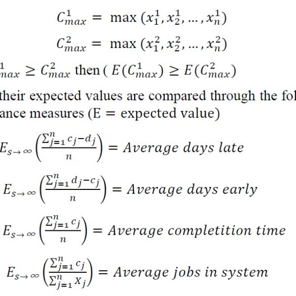
In addition, the total cost is calculated considering the Holding Cost ( ), which is the cost of keeping a unit in inventory, and the Penalty Cost ( ), the cost of not delivering a unit on time. Then, the expected value of the costs is given by

3.2.  Method case study

To exemplify the analysis method, the following case is proposed. Let suppose a robot that receives six jobs simultaneously and whose processing time corresponds to a normal distribution, with a mean, a standard deviation, and a known delivery date for each job. It is intended to minimize the total time of early and late production, and consequently, the total cost associated with holding inventory and penalties from customers. Likewise, it is considered that the robot has no setup interruptions during the processing of the six jobs and that the holding and penalty cost per unit are both the same for all the jobs.

The method to perform the sensitivity analysis of the total cost is based on the construction of a simulator of production runs with stochastic processing times, which receives the following inputs:

• A set of six jobs that arrive simultaneously.
• A mean and a standard deviation for the processing time of each job, assuming that the times follow a normal distribution.
• A due date for each job.
• An early production inventory holding cost and a late production penalty cost, per piece per day and pervasive for all jobs.
• As an example, the following parameters of the problem to perform the simulation are considered.

Table 2: Parameters used in the simulation of production runs. Own elaboration.

Job	Average (days)	Standard deviation (days)	Probability distribution	Due date
				(days)
A	4	1	Normal	34
B	10	1	Normal	25
C	2	0.5	Normal	18
D	14	1	Normal	30
E	12	1	Normal	14
F	6	1	Normal	22

Given the above parameters, the stochastic processing times are simulated through an inverse normal distribution function, whose calculation involves a random probability variable. Subsequently, the sequencing of jobs is performed in the robot based on the dispatch rules First Come First Served (FCFS), Shortest Processing Time (SPT), Longest Processing Time (LPT) and Earliest Due Date (EDD). Finally, the total cost of the system per rule is obtained, whose calculation is the sum of the cost of keeping the early jobs in inventory and the penalty cost of the late jobs. This algorithm is presented in Figure 1, since it is not proving a theorem, perhaps with other examples the solution could change, but the algorithm of analysis is the same.

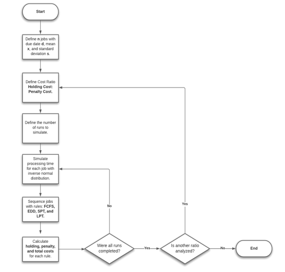
Figure 1: Algorithm to simulate production runs with stochastic processing times. Own elaboration

As the next step in the analysis, the behavior of the total cost of each rule with respect to the three cases of the Holding Cost – Penalty Cost relationship will be identified in such a way that the runs will be carried out as: 1) Holding Cost will be defined at $4 and the Penalty Cost at $2 for the case greater than; 2) $2 and $4 for the case less than; and 3) $3 and $3 for the case equal to. Once it has been verified if the cases of the Holding Cost – Penalty Cost relationship affect the total cost of the rules, then the degree of the sensitivity will be analyzed in each of the cases that were significant. To do this, the holding cost will be varied in a range of values ​​between $ 1 and $ 500, while the penalty cost is fixed at $ 1. Subsequently, the penalty cost will be varied in the same range, while the holding cost remains fixed at $1. This sensitivity analysis of the total cost of the system will be carried out for each of the rules. Thus, the objective of this method is to observe how the total cost of the system changes when the following factors change: the sequencing rule used, the cases of the Holding Cost – Penalty Cost relationship, and the ratio between these costs (for example, $5 of Holding Cost and $1 of Penalty Cost is a 5:1 ratio). It is important to mention that a previous work deals with a scheduling model taking in account earliness/tardiness penalties [35], along with fuzzy processing times, but without considering the Holding Cost Penalty Cost ratio.

4. Results

4.1.  Analysis of the holding cost – penalty cost relationship use

To begin with, it is important to analyze the three cases that could occur in the unit cost relationship per day for early and late production presented before: Identifying the behavior of the total cost of the system for each of these three cases will allow to define if the change in the Holding Cost – Penalty Cost relationship is significant for the selection of sequencing rules in terms of the total cost.

In the first place, the behavior of the total cost is analyzed for the three cases of relationship Holding Cost – Penalty Cost; for which, the following runs were carried out in the simulator.

• 100 runs for the case Holding Cost = Penalty Cost in a 1:1 ratio
• 100 runs for the case Holding Cost > Penalty Cost in a 2:1 ratio
• 100 runs for the case Holding Cost < Penalty Cost in a 1:2 ratio

Table 3: Results of the relevant parameters of each dispatch rule for each case of the Holding Cost – Penalty Cost relationship. Own elaboration.

Case	Parameters	FCFS	EDD	SPT	LPT
Holding Cost = Penalty Cost	Total Cost	(294.11, 298.4)	(119.4, 124.9)	(283.3, 287.7)	(291.4, 303.1)
	Average days early	(7.26, 7.58)	(1.31,1.51)	(9.55 9.86	(2.44,2.63)
	Average days late	(8.84 9.21)	(5.17,5.57)	(6.02,6.31)	(13.66,16.3)
	Average completion time (min)	(25.11 25.75)	(27.51,28.0)	(20,20.56)	(34.95,38.5)
	Average jobs in system	(3.18, 3.22)	(3.48, 3.52)	(2.53, 2.57)	(4.42, 4.46
Holding Cost < Penalty Cost	Total Cost	(302.7, 308.43)		(262.8, 267.9)	(358, 373.8)
			(143.99, 151.7)
	Average days early	(7.155 7.44)	(1.26,1.46))	(9.39 9.66)	(2.40, 2.61)
	Average days late	(8.91, 9.24)	(6.15, 6.43)	(6.15, 6.43)	(13.67,14.3)
	Average completion time (min)	(25.32, 25.9)	(27.68 28.22)	(20.3, 20.8)	(34.9, 35.6)
	Average jobs in system	(3.18969, 3.22358)	(3.48454, 3.51598)	(2.56231, 2.59381)	(4.40619, 4.43769)
Holding Cost > Penalty Cost	Total Cost	(281.5, 285.3)	(98.3, 101.8)	(301.8, 306.3)	(224.96, 234.21)
	Average days early	(7.01, 7.31	(1.31, 1.51)	(9.41, 9.63)	(2.3596, 2.5765)
	Average days late	(9.054, 9.363)	(5.33, 5.704)	(6.16, 6.43)	(13.9,  14.5)
	Average completion time (min)	(25.59, 26.07)	(27.67,28.21)	(20.39,20.8)	(35.25,  35.87)
	Average jobs in system	(3.20,3.23)	(3.4, 3.49)	(2.55, 2.58)	(4.41, 4.44)

It is necessary to mention that 40 runs are enough to have accurate results, but 100 are made to ensure their reliability. The simulator obtains the average value of all the runs for the following parameters in each rule: total cost, average days early, average days late, average completion time and average jobs in the system. Although the parameter of interest is the total cost, it is relevant to identify the behavior of the other parameters for each rule in each case of the relationship. Confidence intervals were made at 95% reliability, in every sample it was tested if the data were adjusted to a normal distribution, since the population variance was not known, the student’s t-distribution was used [36]. The results of the analysis are shown in Table 3.

The interpretation of the results of this analysis is as follows:

• As can be seen, the magnitude of the total cost presents variations from one case to another in each rule, which will be studied in detail in the next section when carrying out the sensitivity analysis of the total cost in each case. For now, it is relevant to note that the performance of the sequencing rules does change depending on the case in which the cost relationship is found.
• In this sense, in the Holding Cost = Penalty Cost case and the Holding Cost < Penalty Cost case the same effect is observed when the order of the sequencing rules is analyzed in terms of total cost and even in the terms of the other parameters. For both cases the order of the sequencing rules from lowest to highest cost is: EDD, SPT, FCFS and LPT. However, the performance of the rules changes for the Holding Cost > Penalty Cost case, since the order of these rules from lowest to highest cost is EDD, LPT, FCFS and SPT.
• Given the above, it can be established that the three cases of the relationship Holding cost – Penalty cost identified can be grouped into only two significant cases for the selection of sequencing rules according to their performance: Holding cost > Penalty cost and Holding cost Penalty cost.
• Optimal rule: In any case of the Holding Cost – Penalty Cost relationship, the rule that generates the lowest total cost is EDD; this is because this rule minimizes the average earliness time and the average tardiness time in all cases.
• Most expensive rule: This rule depends on the two significant cases identified:

1)     When the Holding cost   Penalty cost, the rule with the worst performance in terms of the total cost is LPT. This is because LPT is associated with the highest average completion times; therefore, this results in the highest delay times of the four sequencing rules.

2)       When Holding Cost > Penalty Cost the worst-performing rule is SPT. This is because SPT is associated with the lowest average completion times; therefore, this results in the highest early times of the four sequencing rules.
4.2.  Sensitivity analysis of the total cost

As shown in the previous analysis, there are only two significant cases of the relationship Holding cost – Penalty cost for the selection of sequencing rules. Due to this, the sensitivity analysis of the total cost will be applied with respect to these two cases for each of the four rules studied. The objective is to vary one of the two costs while the other remains fixed to change the ratio and visualize the effect of this change on the total cost when their relationship is found in one case or another.

In the first place, the case Holding Cost > Penalty Cost is analyzed, performing the following runs on the simulator:

• 100 runs for the Holding Cost > Penalty Cost in a 5:1 ratio
• 100 runs for the Holding Cost > Penalty Cost in a 10:1 ratio
• 100 runs for the Holding Cost > Penalty Cost in 50:1 ratio
• 100 runs for the Holding Cost > Penalty Cost in a 100:1 ratio
• 100 runs for the Holding Cost > Penalty Cost case in a 500:1 ratio

As shown, there are runs for cases where Holding Cost is 5 times greater than Penalty Cost, 10 times greater, 50 times greater, etc. It is worth mentioning that in a practical approach a very large ratio may be unrealistic, but it was analyzed for experimental purposes. Table 4 shows the average total costs of each sequencing rule with respect to each of the simulated ratios; in the same way, in Figure 2 these results were graphed by rule.

Table 4: Average total cost per sequencing rule for each ratio of the Holding Cost > Penalty Cost case. Own elaboration.

Holding Cost: Penalty Cost Ratio	Quotient	Average Total Cost
		FCFS	EDD	SPT	LPT
05:01	5	274.47	73.21	323.3	157.63
10:01	10	493.38	111.73	612.87	221.32
50:01:00	50	2,240.00	423.12	2,884.80	837.49
100:01:00	100	4,393.56	835.98	5,719.99	1,594.16
500:01:00	500	22,155.67	4,042.66	28,723.70	7,850.70
Slope		44.2324	8.0252	57.3925	15.5683

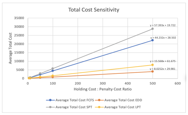
Figure 2: Sensitivity of the average total cost with respect to the costs ratio for the Holding Cost > Penalty Cost case. Own elaboration

To obtain the equations in Figure 2 a simple linear regression was performed for each rule, in which the total cost was used as the response variable and the Holding Cost: Penalty Cost ratio as the explanatory variable, whose regression model is the following:

The parameters  and  were estimated with the least-squares method in order to define a line that fits the data by minimizing the sum of squares of the regression errors [34]. In particular, the estimation of the parameter  represents the slope of the line or in this case, the degree of sensitivity of the total cost with respect to the change in the Holding Cost: Penalty Cost ratio.

The above evidence shows that with a higher holding cost, the total cost grows linearly at different speeds according to the applied sequencing rule. According to the slopes obtained in the regression of the data, it is noted that the least sensitive rule is EDD increasing $ 8.03 for each unit that increases the Holding Cost: Penalty Cost ratio, while the most sensitive rule is SPT increasing $ 57.39 per each unit that increases that ratio. That is, when Holding Cost > Penalty Cost the SPT rule is 7.15 times more sensitive than EDD; the other sensitivity relationships between rules are found in Table 5. Likewise, a grouping between the rules is observed, with EDD and LPT being notoriously less sensitive than FCFS and SPT for this case.

Table 5: Sensitivity relationships between the sequencing rules for the Holding cost > Penalty cost. Own elaboration.

Case: Holding Cost > Penalty cost
Rule sensitivity:	Regarding the rule:
	EDD	LPT	FCFS	SPT
SPT	7.15	3.69	1.3	–
FCFS	5.51	2.84	–
LPT	1.94	–
EDD	–

Second, the case Holding Cost  Penalty Cost is analyzed, performing the following runs on the built simulator:

• 100 runs for the Penalty Cost case Holding Cost in a 1:1 ratio
• 100 runs for the Penalty Cost caseHolding Cost in 5:1 ratio
• 100 runs for the Penalty Cost case Holding Cost in a 10:1 ratio
• 100 runs for the Penalty Cost case Holding Cost in 50:1 ratio
• 100 runs for the Penalty Cost case Holding Cost in a 100:1 ratio
• 100 runs for the Penalty Cost case Holding Cost in 500:1 ratio

It is worth mentioning that for the analysis of this case, the Holding Cost – Penalty Cost relationship was inverted to obtain an integer ratio comparable to the previous case. In this context, Table 6 shows the average total costs of each sequencing rule for each of the simulated ratios and in Figure 3 the data plotted by rule is presented.

Table 6: Average total cost per sequencing rule for each ratio of the Holding Cost  Penalty Cost case. Own elaboration.

Penalty Cost: Holding Cost	Quotient	Average Total Cost
Ratio		FCFS	EDD	SPT	LPT
01:01	1	98.71	40.84	95.29	99.65
05:01	5	314.92	170.44	244	432.55
10:01	10	593.02	339.96	434.08	855.11
50:01:00	50	2,771.24	1,643.66	1,921.44	4,231.30
100:01:00	100	5,584.92	3,381.25	3,872.48	8,635.48
500:01:00	500	27,703.64	16,749.71	19,236.98	42,487.58
Slope		55.3371	33.4991	38.3847	84.957

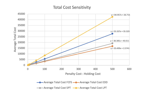
Figure 3: Sensitivity of the average total cost with respect to the cost ratio for the Holding Cost   Penalty Cost case. Own elaboration

As in the previous analysis, the parameters  and  of the regression equations in Fig. (3) were estimated through the least-squares method, where  is the parameter that represents the degree of sensitivity of the total cost with respect to the change in Holding Cost: Penalty Cost ratio for each rule.

For this case, it can be interpreted that the higher the Penalty Cost is, the total cost grows linearly with different slopes depending on the dispatch rule implemented, similar to the previous case. Again, the least sensitive rule is EDD with an increase of $33.50 for each unit that increases the Penalty Cost: Holding Cost ratio, while the most sensitive rule is LPT with an increase of $ 84.96 for each unit that increases the ratio. Being then 2.54 times more sensitive LPT than EDD when Holding Cost <= Penalty Cost. Like the previous analysis, the other sensitivity relationships between rules for this case are found in Table 7. Furthermore, the EDD and SPT rules have a similar sensitivity in both cases: Holding Cost > Penalty Cost case and Holding Cost  Penalty Cost case.

Table 7: Sensitivity relationships between the sequencing rules for the Holding cost <= Penalty cost. Own elaboration.

Case: Holding Cost    Penalty Cost
Rule sensitivity:	Regarding the rule:
	EDD	SPT	FCFS	LPT
LPT	2.54	2.21	1.54
FCFS	1.65	1.44
SPT	1.15
EDD

Once the analysis has been carried out for both cases, it is possible to reach the following conclusions:

• As demonstrated, a sequencing rule can present different degrees of sensitivity depending on in which of the two significant cases of the Holding Cost – Penalty Cost relationship this rule is found. For example, EDD is the optimal rule in terms of total cost for all the proportions. However, it presents a lower sensitivity and the lowest total costs when it is in the Holding Cost > Penalty Cost case than when it is in the Holding Cost Penalty Cost case, as shown in Figure 4.
• In the Holding Cost <=Penalty Cost case, EDD is the rule that has the lowest total cost (RQ1) however SPT is the rule that is less sensitive to cost variation as can be seen in Fig 4 (RQ2).
• Furthermore, it can be observed in Figure 4 that all the rules are less sensitive in the Holding Cost> Penalty Cost case, except the SPT rule which is less sensitive in the Holding Cost Penalty Cost case (RQ2).
• That is, when the total cost is the parameter to optimize in a changing environment, it is not only possible to choose the most economical sequencing rule, but it is also convenient to look for a Holding Cost – Penalty Cost relationship that provides less sensitivity to changes of those costs. This will not only ensure lower-cost production but will also allow the production system to respond more robustly to changes in the economic environment in this case the less sensitive is SPT rule.

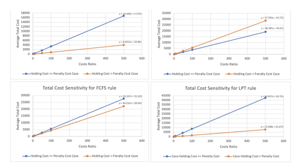
Figure 4: Comparison of the sensitivity of the total cost for each case of the Holding Cost – Penalty Cost relationship by sequencing rule, own elaboration

• Furter, in Appendix A, the parameters of the simulation run where different Holding Cost – Penalty cost relationships are handled, the EDD is the rule that generates the lowest costs (RQ1), however if they are compared with the standard deviation, the STP it is the most robust or the one with the least variation in costs (RQ2).

5. Discussion

Based on the obtained results, this section studies the applicability of the sensitivity analysis of the total cost of the sequencing rules within organizations that manufacture under an agile approach. This study starts from the fact that sequencing rules are applied in a changing environment that constantly causes a variation in the penalty costs of late production and the holding costs of early production. Due to the above, it is relevant to point out how these costs could vary and how the sensitivity analysis could help make better decisions.

Consider the following numerical example to demonstrate the variation of penalty costs in a changing environment:

• During the negotiations of a manufacturing organization with a customer, it was determined as a policy that after the first 5 days of delay, a penalty of 2% of the volume value of the parts will be paid for each additional day of a delay; considering 5 business days in a week. It is not allowed to exceed 45% of the value of the pieces and in case of exceeding it, the contract will be canceled.
• Consider that the value of each piece is $100 and that the manufacturing company must make quarterly deliveries of batches that vary in size from period to period, due to changing customer requirements.
• Suppose that this quarter the company delivers a batch of 1,000 pieces 10 days late, so the penalty would be 5% of the total value of $ 100,000; that is, $5,000 would be paid. As result, the unit penalty cost is $5 for each piece of this batch delayed 10 days; therefore, the penalty cost for each piece per day is $0.5.
• The following quarter, the company delivers a batch of 2000 pieces 25 days late, which implies a penalty of 20% of the total value of $200,000; that is $40,000. Thus, the unit penalty cost of $20 for each piece is delayed 25 days; therefore, the penalty cost for each piece per day is $0.8.
• Now consider that the next period, the company delivers a batch of 3,000 pieces 25 days late as well; that is, again 20% of the total value of the lot amounting to $ 300,000. This means that a penalty of $60,000 will be paid, the penalty unit cost also being $20 for each piece delayed 25 days; hence, the penalty cost for each piece per day returns to $0.8.
• Then it is observed that the penalty cost per product does not depend on the volume of late parts, as shown in the second and third quarters of the example. The lot size can vary, but if the number of days late is kept constant, arithmetically the penalty unit cost will always be the same.
• Given the above, it can be established that the unit penalty cost depends directly on the number of days of delay, for a policy like the one used in this example. However, it should be noted that variations in batch sizes could affect this cost indirectly, as larger, and fluctuating batches may require more time to complete and deliver.

On the other hand, there are multiple works that propose various mathematical models to calculate the Cost of Maintaining the inventory [37,38]. However, more works agree that the traditional method is to establish this cost as a percentage of the value of the product and keep it constant for each item and for each unit of time. In fact, in the literature, it is mentioned that this percentage ranges between 12% and 34% of the value of the product, or a reference to similar organizations, or an industry average is used [39,40]. Although previous works point out that the traditional method has deficiencies to adequately estimate the Cost of Maintaining the inventory in practice, this approach is commonly found [41].  Due to the above and for the sake of simplicity, the traditional method is used to exemplify the Holding cost variance in a changing environment, although the exercise could be adapted to a mathematical model with greater precision.

To understand the variation of Holding Cost in a constantly changing environment, consider the following example:

• Continuing with the situation raised above, the manufacturing company offers the basic model of its product at $ 100 per piece. However, customer requirements tend to vary from one period to another and they request parts with additional finishes and machining, larger dimensions, different materials, etc. This changes the manufacturing cost and, therefore, the value of the product.
• Consider that the company has taken a traditional approach to define its Holding cost based on an industry average, representing 25% of the value of its product.
• In this sense, its base model has an annual inventory cost of $ 25 for each part. Considering that the company works 260 days a year, there is a holding cost per piece per day of $ 0.1 for the base model.
• Suppose that in the first quarter of the year, the customer ordered a batch of parts with additional machining and larger dimensions, increasing the value of the product by $200 per part. Since 25% of the product value is held fixed, these parts have an annual inventory cost of $ 50 for each part and an inventory cost per part per day of $ 0.2 for this special specification model.
• In this way, the Holding cost increases proportionally to the value of the product, which is reasonable considering that a more valuable product may incur higher risk costs (such as obsolescence or damage), space costs, service costs (such as insurance or taxes) and even capital costs [13].

Variations in holding and penalty costs may be subject to other factors in addition to those described above. Nonetheless, in this study these conditions will be used to explain how the decision-maker could use sensitivity analysis to control and ensure the agility of the manufacturing system at a low cost. As an example, a tool was built in Excel that allows calculating the maximum number of days that a batch can be delayed to keep the Penalty Cost below the holding cost and thus remain in the case it presents lower sensitivity of the total cost with respect to the variations of these two costs. This calculator is based on the penalty policy that was described in this section and through the Solver tool, the maximum value of days of delay is found that meets the restriction Holding Cost > Penalty Cost.

In Figure 5 the tool built is shown, assuming that for a certain quarter there is a Holding Cost of $ 0.80 per piece per day and the values defined in the penalty policy described above are used. As can be seen, the calculator determines that the delivery of that batch cannot be more than 24 days late, so that the Penalty Cost does not equal or exceed $0.80.

As explained in previous sections, EDD is the optimal sequencing rule to use when the total cost is the parameter to minimize. However, in a changing environment characterized mainly by the variation of customer requirements, in Agile Manufacturing, it is necessary to look for a Holding Cost – Penalty Cost relationship that provides greater robustness to the variations of these two costs. Through the sensitivity analysis of the total cost of the sequencing rules, it was shown that the SPT rule is more robust in terms of cost (RQ2) although EDD has the less cost (RQ1); therefore, it is convenient that the Penalty Cost can be kept varying below the Holding Cost. Otherwise, it is necessary to shorten delivery times through different Lean techniques, production planning and control, work-study, set-up time reduction techniques, theory of restrictions, etc. [42].

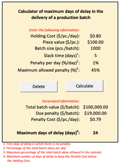
Figure 5: Calculator that determines the maximum number of days of delay to keep the Penalty Cost below the Holding Cost. Own elaboration

6. Conclusions

This article presents a sensitivity analysis that serves as an instrument to take decisions in the selection of sequencing rules when inventory maintenance and penalty costs vary in a changing environment, with the objective of reducing the total cost and to be prepared if costs vary like in Agile Manufacturing. Speaking about agile manufacturing, recent works propose the sequencing and dispatch method for facilities where humans and robots are mixed, while handling uncertainty in process times. However, these works do not present a cost sensitivity analysis; the total cost as performance metrics allows to control and ensure an agile manufacturing system in a changing environment.

The problem of the study are jobs that are to be handled by robots whose processing times follow a normal distribution with known mean and standard deviation, and that sometimes need to be handled by humans to meet customer requirements. Delivery dates are also known. The objective is to minimize the total time of early and late production, and consequently, the total cost associated with keeping the inventory and penalties from customers. Jobs are sequenced in the robot based on FCFS, SPT, LPT y EDD dispatch rules. Finally, the total cost of the system per rule is obtained, whose calculation is the sum of the cost of keeping the early jobs in inventory and the penalty cost of the late jobs.

In order to carry out the sensitivity analysis by a rule, first the effect on the total cost of the three identified cases of the Holding Cost – Penalty Cost relationship was analyzed. After verifying that this relationship was significant for the performance of the rules, in each case the Holding Cost was varied, while the Penalty Cost was fixed and vice versa. In this sensitivity analysis, it was observed how the total cost of the system changes when the following factors vary: the sequencing rule used, the case of the Holding Cost – Penalty Cost relationship, and the ratio between both costs.

It was observed that when Holding Cost = Penalty Cost and Holding Cost < Penalty Cost, the same effect occurred in the order of the sequencing rules in terms of the total cost. In this sense, for both cases, the order of the sequencing rules from lowest to highest cost is EDD, SPT, FCFS and LPT. On the other hand, for the case Holding Cost > Penalty Cost, the order of the rules EDD is the best in terms of cost (RQ1); but the SPT rule is the is the most robust rule with respect to cost ratio (RQ2), no matter if HC>PC or PC<=HC.

Subsequently, the degree of the sensitivity of each rule regarding the movement of costs is analyzed. It can be concluded that a dispatch rule may have different degrees of sensitivity depending on which of the two significant cases of the Holding – Penalty costs relationship that rule is. For example, EDD is the optimal rule in terms of the total cost for all cases; however, it has lower sensitivity and lower total costs when it is in the case of Holding Cost > Penalty Cost than when it is in the case of Holding Cost  Penalty Cost. Therefore, when the total cost is the parameter to be optimized in a changing environment, it is not only possible to choose the most economical sequencing rule, but also to look for a Holding Cost – Penalty Cost relationship that gives less sensitivity to changes in costs in this case the SPT rule.

Likewise, the applicability of the presented analysis was verified. As a result, a situation was exemplified in which the Holding Cost and the Penalty Cost vary due to changes in customer requirements, either in terms of specifications or volumes requested. Finally, an Excel calculator was built based on the proposed penalty policy. With this tool, the decision-maker can estimate the maximum number of days that the delivery of a batch can be delayed to keep the Penalty Cost below the Holding Cost and, thus, maintain the cost ratio in the case with less sensitivity to total cost; through the sensitivity analysis of the total cost of the sequencing rules, it was shown that the EDD rule is the least in cost, but the SPT is the most robust. Therefore, it is convenient that the Penalty Cost is kept varying below the Holding Cost. As a result, it is shown that the present sensitivity analysis can provide tools for decision making with the objective of reducing costs in a volatile environment like Agile Manufacturing. Future work includes running the simulation with stochastic processing times for 2 or more robots and performing cost sensitivity analysis.

1. A. Ghasemi, A. Ashoori, C. Heavey, “Evolutionary Learning Based Simulation Optimization for Stochastic Job Shop Scheduling Problems,” Applied Soft Computing, 106, 107309, 2021, doi:10.1016/j.asoc.2021.107309.
2. P. Sharma, A. Jain, “Performance analysis of dispatching rules in a stochastic dynamic job shop manufacturing system with sequence-dependent setup times: Simulation approach,” CIRP Journal of Manufacturing Science and Technology, 10, 110–119, 2015, doi:10.1016/J.CIRPJ.2015.03.003.
3. M.A. Şahman, “A discrete spotted hyena optimizer for solving distributed job shop scheduling problems,” Applied Soft Computing, 106, 107349, 2021, doi:10.1016/J.ASOC.2021.107349.
4. Pinedo Michael L., Scheduling, 5th ed., Springer Science, New York, 2016.
5. Z. Shi, S. Gao, J. Du, H. Ma, L. Shi, “Automatic Design of Dispatching Rules for Real-time optimization of Complex Production Systems,” Proceedings of the 2019 IEEE/SICE International Symposium on System Integration, SII 2019, 55–60, 2019, doi:10.1109/SII.2019.8700391.
6. B. Maskell, “The age of agile manufacturing,” Supply Chain Management, 6(1), 5–11, 2001, doi:10.1108/13598540110380868/FULL/XML.
7. F. Maciá Pérez, J.V. Berna-Martinez, D. Marcos-Jorquera, I. Lorenzo Fonseca, A. Ferrándiz Colmeiro, “Cloud agile manufacturing,” IOSR Journal of Engineering, 2, 1045–1048, 2012.
8. N.G. Hall, M.E. Posner, “Sensitivity Analysis for Scheduling Problems,” Journal of Scheduling 2004 7:1, 7(1), 49–83, 2004, doi:10.1023/B:JOSH.0000013055.31639.F6.
9. D.R. Anderson, D. Sweeney, T.A. Williams, Contemporary Management Sciences with Spreadsheets, South Western College Publishing, Cincinatti OH, 1999.
10. T. Danaci, D. Toksari, “A branch-and-bound algorithm for two-competing-agent single-machine scheduling problem with jobs under simultaneous effects of learning and deterioration to minimize total weighted completion time with no-tardy jobs,” International Journal of Industrial Engineering: Theory, Applications, and Practice, 28(6), 577–593, 2022, doi:10.23055/ijietap.2021.28.6.7723.
11. A.W.J. Kolen, A.H.G. Rinnooy Kan, C.P.M. van Hoesel, A.P.M. Wagelmans, “Sensitivity analysis of list scheduling heuristics,” Discrete Applied Mathematics, 55(2), 145–162, 1994, doi:10.1016/0166-218X(94)90005-1.
12. Y.N. Sotskov, “Stability of an optimal schedule,” European Journal of Operational Research, 55(1), 91–102, 1991, doi:10.1016/0377-2217(91)90194-Z.
13. S.A. Kravchenko, Y.N. Sotskov, F. Werner, “Optimal schedules with infinitely large stability radius ∗,” Http://Dx.Doi.Org/10.1080/02331939508844080, 33(3), 271–280, 2007, doi:10.1080/02331939508844080.
14. R.L. Graham, E.L. Lawler, J.K. Lenstra, A.H.G.R. Kan, “Optimization and Approximation in Deterministic Sequencing and Scheduling: a Survey,” Annals of Discrete Mathematics, 5(C), 287–326, 1979, doi:10.1016/S0167-5060(08)70356-X.
15. C.A. Tovey, “A Simplified Anomaly and Reduction for Precedence Constrained Multiprocessor Scheduling,” Http://Dx.Doi.Org/10.1137/0403051, 3(4), 582–584, 2006, doi:10.1137/0403051.
16. A. Wagelmans, Sensitivity analysis in Combinatorial Optimization, Erasmus University, Rotterdam, Netherlands, 1990.
17. P. Kouvelis, G. Yu, A Robust Discrete Optimization Framework, Springer, Boston, MA: 26–73, 1997, doi:10.1007/978-1-4757-2620-6_2.
18. R.L. Daniels, P. Kouvelis, “Robust Scheduling to Hedge Against Processing Time Uncertainty in Single-Stage Production,” Http://Dx.Doi.Org/10.1287/Mnsc.41.2.363, 41(2), 363–376, 1995, doi:10.1287/MNSC.41.2.363.
19. P. Kouvelis, R.L. Daniels, G. Vairaktarakis, “Robust scheduling of a two-machine flow shop with uncertain processing times,” IIE Transactions 2000 32:5, 32(5), 421–432, 2000, doi:10.1023/A:1007640726040.
20. F.S. Hillier, G.J. Lieberman, Introduction to Operations Research, 9th ed., McGraw Hill, New York, 2010.
21. X. Liu, W. Li, “Approximation Algorithm for the Single Machine Scheduling Problem with Release Dates and Submodular Rejection Penalty,” Mathematics 2020, Vol. 8, Page 133, 8(1), 133, 2020, doi:10.3390/MATH8010133.
22. M. Kühn, M. Völker, T. Schmidt, “An Algorithm for Efficient Generation of Customized Priority Rules for Production Control in Project Manufacturing with Stochastic Job Processing Times,” Algorithms 2020, Vol. 13, Page 337, 13(12), 337, 2020, doi:10.3390/A13120337.
23. C. Te Yang, “An inventory model with both stock-dependent demand rate and stock-dependent holding cost rate,” International Journal of Production Economics, 155, 214–221, 2014, doi:10.1016/J.IJPE.2014.01.016.
24. H. Ding, M. Schipper, B. Matthias, “Optimized task distribution for industrial assembly in mixed human-robot environments – Case study on IO module assembly,” IEEE International Conference on Automation Science and Engineering, 2014-January, 19–24, 2014, doi:10.1109/COASE.2014.6899298.
25. M. Messner, F. Pauker, G. Mauthner, T. Frühwirth, J. Mangler, “Closed Loop Cycle Time Feedback to Optimize High-Mix / Low-Volume Production Planning,” Procedia CIRP, 81, 689–694, 2019, doi:10.1016/J.PROCIR.2019.03.177.
26. O. Cardin, D. Trentesaux, A. Thomas, P. Castagna, T. Berger, H. Bril El-Haouzi, “Coupling predictive scheduling and reactive control in manufacturing hybrid control architectures: state of the art and future challenges,” Journal of Intelligent Manufacturing 2015 28:7, 28(7), 1503–1517, 2015, doi:10.1007/S10845-015-1139-0.
27. D. Ivanov, A. Dolgui, B. Sokolov, “Robust dynamic schedule coordination control in the supply chain,” Computers & Industrial Engineering, 94, 18–31, 2016, doi:10.1016/J.CIE.2016.01.009.
28. A. Cataldo, A. Perizzato, R. Scattolini, “Production scheduling of parallel machines with model predictive control,” Control Engineering Practice, 42, 28–40, 2015, doi:10.1016/J.CONENGPRAC.2015.05.007.
29. A. Casalino, A.M. Zanchettin, L. Piroddi, P. Rocco, “Optimal Scheduling of Human-Robot Collaborative Assembly Operations With Time Petri Nets,” IEEE Transactions on Automation Science and Engineering, 70–84, 2019, doi:10.1109/TASE.2019.2932150.
30. J. Dörmer, H.O. Günther, R. Gujjula, “Master production scheduling and sequencing at mixed-model assembly lines in the automotive industry,” Flexible Services and Manufacturing Journal 2013 27:1, 27(1), 1–29, 2013, doi:10.1007/S10696-013-9173-8.
31. J.T. Lin, C.C. Chiu, Y.H. Chang, “Simulation-based optimization approach for simultaneous scheduling of vehicles and machines with processing time uncertainty in FMS,” Flexible Services and Manufacturing Journal 2017 31:1, 31(1), 104–141, 2017, doi:10.1007/S10696-017-9302-X.
32. U. Saif, Z. Guan, L. Zhang, F. Zhang, B. Wang, J. Mirza, “Multi-objective artificial bee colony algorithm for order oriented simultaneous sequencing and balancing of multi-mixed model assembly line,” Journal of Intelligent Manufacturing 2017 30:3, 30(3), 1195–1220, 2017, doi:10.1007/S10845-017-1316-4.
33. M.D. Rossetti, Simulation Modeling and Arena, 2nd ed., Wiley & Sons, Hoboken, New Jersey, 2015.
34. S. Vinga, J.S. Almeida, “Rényi continuous entropy of DNA sequences,” Journal of Theoretical Biology, 231(3), 377–388, 2004, doi:10.1016/J.JTBI.2004.06.030
35. M.H. Seyyedi, A.M.F. Saghih, Z.N. Azimi, “A FUZZY MATHEMATICAL MODEL FOR MULTI-OBJECTIVE FLEXIBLE JOB-SHOP SCHEDULING PROBLEM WITH NEW JOB INSERTION AND EARLINESS/TARDINESS PENALTY,” International Journal of Industrial Engineering: Theory, Applications, and Practice, 28(3), 2021, doi:10.23055/ijietap.2021.28.3.7445.
36. D.C. Montgomery, G.C. Runger, Applied Statistics and Probability for Engineers, John Wiley & Sons, Inc., New York, 2003.
37. C. Te Yang, “An inventory model with both stock-dependent demand rate and stock-dependent holding cost rate,” International Journal of Production Economics, 155, 214–221, 2014, doi:10.1016/J.IJPE.2014.01.016.
38. V. Pando, J. García-Laguna, L.A. San-José, J. Sicilia, “Maximizing profits in an inventory model with both demand rate and holding cost per unit time dependent on the stock level,” Computers & Industrial Engineering, 62(2), 599–608, 2012, doi:10.1016/J.CIE.2011.11.009.
39. P. Berling, “Holding cost determination: An activity-based cost approach,” International Journal of Production Economics, 112(2), 829–840, 2008, doi:10.1016/J.IJPE.2005.10.010.
40. D.M. Lambert, J.R. Stock, L.M. Ellram, Fundamentals of Logistics Management , McGraw-Hill Higher Education, 1998.
41. R. Chase, R. Jacobs, N. Alquilano, Administración de Operaciones, 12th ed., McGraw-Hill Education, México , 2009.
42. A.H. Alad, V.A. Deshpande, “A Review of Various Tools and Techniques for Lead Time Reduction,” International Journal of Engineering Development and Research, 2, 1159–1164, 2014.

(Click Here)