1. Introduction

In the last decade, we have observed the fast-growing consumption of persistent storage used to implement operational and analytical databases [1]. While the databases become larger, the total number of database applications also continuously increases and the applications themselves, especially the analytical ones, become more sophisticated and advanced than before [2]. Such trends increase the pressure on hardware resources for data processing, particularly on high-capacity and fast persistent storage devices.

Usually, the financial constraints invalidate the single-step replacements of all available persistent storage devices with better ones. Instead, a typical strategy is based on the continuous and systematic replacements of persistent storage devices with only a few at a time. Also, from an economic point of view, it is not worth investing significant funds in faster and larger persistent storage devices when only some of the available data is frequently processed. In reality, only some data sets are accessed more frequently than others. Financial and data processing requirements lead to the simultaneous utilization of persistent storage devices of different speeds and capacities. Therefore, data is distributed over many different storage devices with various capacity and speed characteristics [3]. This leads to a logical model of the multi-tiered organization of persistent storage [4, 5]. The lower tiers (levels) consist of higher capacity and slower persistent storage devices than the lower capacity and faster devices at the higher levels.

Several research works have been already performed on the automatic allocation of storage resources over multi-tiered persistent storage devices and multi-tier caches. For example, in one of the solutions, persistent storage can be allocated over several cache tiers and in different arrangements [6]. Another research work shows how to distribute data on disk storage in the multi-tier hybrid storage system (MTHS) [7].

A number of approaches schedule the allocation of resources over multi-tiered persistent devices based on future predicted workloads. The algorithms for an optimal allocation of persistent storage on multi-tiered devices in environments where future workloads can be predicted have been proposed in [8, 9]. These algorithms arrange data according to an expected workload and contribute to the automated performance tuning of database applications. Most of the existing research outcomes show that performance tuning with the predicted database workloads improves performance during processing time and reduces database administration time [10].

A logical model of multi-tiered persistent storage consists of several tiers (levels) of persistent storage visible as a single persistent storage container. The processing speeds at the same tier are alike. Each tier is divided into several partitions, where each partition is a logical view of a physical persistent storage device that implements a particular tier. Such a view is compatible with the organization of persistent storage within cloud systems. Nowadays, data can be stored on several remote devices. It contributes to the changes in the working style where the employees can work from home or distance. Therefore, storage on the cloud is required to provide access to data online anywhere, anytime over an internet connection. In addition, cloud storage for organizations must be shared by many users. Therefore, partitioning of persistent storage is required so that users can access storage simultaneously. Also, the efficient management of storage allocation on multi-tiered persistent storage with partitions is an essential factor for the performance of cloud systems.

The illustration of multi-tiered persistent storage with partitions is shown in Figure 1. Typically, the higher tiers of persistent storage have lower capacities and faster access times than the lower tiers. In a physical model, a sample multi-tiered persistent storage consists of the physical persistent storage devices available on the market, such as NVMe, SSD, and HDD [3].

Efficient processing of data stored at multi-tiered persistent storage is an interesting problem. When processed, data can “flow” from lower tiers to free space at the higher tiers to speed-up access to such data in the future. Scheduling the data transfers between the tiers require the allocation/deallocation of data based on the speed and capacities of the tiers. Thus, making the correct scheduling decisions automatically and within a short period of time becomes a critical factor for the overall performance of data processing.

Because of its limited capacity, it is impossible to store all data at the topmost and the fastest tier. Therefore, we must prepare for a compromise between the capacity, speed, and price of available multi-tiered persistent storage. Such compromise leads to all data being distributed over many tiers of multi-tiered persistent storage.

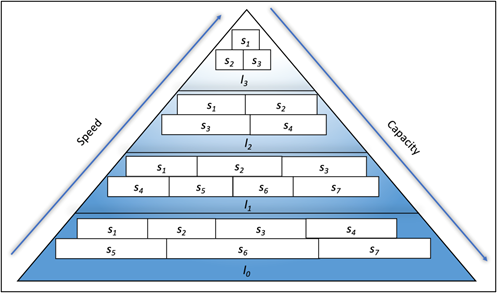
Figure 1: Illustration of multi-tiered persistent storage with four tiers divided into partitions

The main research objective of this work is to speed up data processing in environments where all data is located at multi-tiered persistent storage. We assume that data processing is organized as a collection of pipelines where the outputs from one operation are the inputs to the next operation in a pipeline. A strategy to speed up the data processing in a pipeline is to write the outputs of each operation to the highest available persistent tiers. The benefits of such a strategy are twofold. First, data is written faster at the higher tiers than at the lower ones. Second, the following operation in a pipeline reads input data more quickly from the higher tiers. An essential factor in such a strategy is an optimal release of persistent storage allocated at the higher tiers to store temporary data.

Another problem addressed in the paper is the lower-level optimization of query processing on multi-tiered persistent storage. The present query optimizers do not consider an efficient implementation of higher-level operations on data located at multi-tiered persistent storage. However, it is possible to significantly improve performance by implementing higher-level operations in ways consistent with the characteristics of available persistent storage. Our second research objective is to generate more efficient data processing plans for predicted and unpredicted database workloads through the optimal implementation of elementary operations on data located at multi-tiered persistent storage.

The contributions of the paper are the following. First, the paper shows how to extend and apply a notation of Petri nets to describe the data flows in multi-tiered persistent storage. Second, the paper presents the algorithms that find optimal query processing plans through the linearization of Petri nets. Third, the paper analyses the results of experiments to show that query processing plans generated by the new algorithms efficiently use the properties of multi-tiered persistent storage.

This paper is an extension of work originally presented in [11]. The paper is organized in the following way. Section 2 extends a notation of Petri nets to describe data flow in query processing. Sections 3 and 4 present the algorithms for the automatic allocation of storage available on multi-tiered persistent storage devices. Section 5 describes an experiment, and Section 6 summarizes the paper.

2. Basic Concepts

In this work, we consider a scenario where a database application submits an SQL query to a relational database server. Then, a typical query optimizer finds an optimal query processing plan. Such a plan includes the list of operations organized as a directed bipartite graph. Then, to discover the data flows between the elementary operations, a plan is transformed into an extended Petri Net [12]. Finally, a graphical notation of Petri Nets represents the flow of data when processing a query.

The original Petri net model includes two types of elements: places and transactions. Places are denoted as circles, and transactions are denoted as vertical rectangles. Zero or more tokens, denoted as small black circles, can be located in the places. Arcs are connected between places and transactions—the illustration of Petri Net is shown in Figure 2.

An Extended Petri Net is quadruple <B, E, A, W> where B and E are disjoint sets of places and transitions. Places are visualized as circles, and transitions are visualized as rectangles or bars. Arcs A Í (B × E) È (E × B) connect the places and transitions. A place may contain a finite number of tokens visualized as black circles, or it can be empty. A transition fires depending on the number of tokens connected at the input place. When an input place has no token, a transition is at a waiting state.

In our case, sets of places, B, are interpreted as input/output data sets, and the sets of transitions, E, are interpreted as operations on data sets (see Figure 3 below).

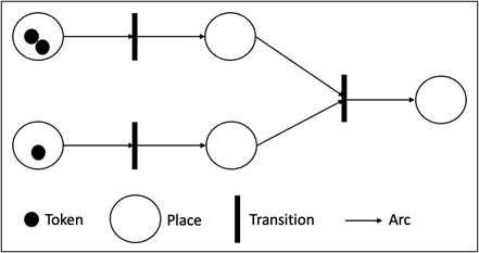
Figure 2: An original sample structure of a Petri net

Arcs, A, determine the input and output data sets of the operations. A weight function W: A→N⁺ determines the estimated total number of data blocks read and written by each operation. See the numbers attached to the arcs in Figure3. The root nodes are the places (data sets) in B that do not have the arcs from the transitions (operations) E. The root nodes represent the input data sets located in a database. An operation can have more than one input and output data set. Likewise, more than one operation can share input and output data sets.

There are two types of persistent storage data sets B: permanent or temporary. Both types of data sets are stored in multi-tiered storage. A temporary data set can be removed from the storage when it is no longer needed.

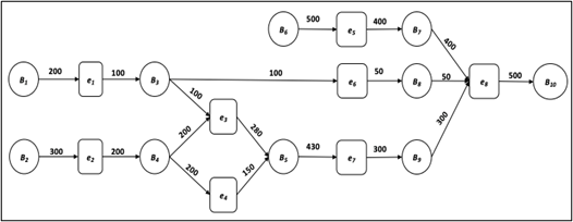
Figure 3: Data processing and data flows represented as an extended Petri net

Let E = {e_i, …, e_j} be a set of operations obtained for a query Q processing plan created by a database query optimizer. Each operation e_i is represented by a pair e_i = ({B_i, …, B_m}, {B_(m+1), …, B_n}), where {B_i, …, B_m} are the input data sets and {B_(m+1), …, B_n} are the output data sets of an operation e_i in E. Some of the input and output data sets processed by an operation e_i are permanent, and some of them are temporary.

This paper focuses on managing the multi-tiered persistent storage efficiently for each input/output data sets of each operation and generates the best allocation plan, called a processing plan, for each query. A list of persistent storage tiers is denoted as a sequence L = <l₀, …, l_n>. We have n+1 tiers where l₀ denotes the lowest tier, called a base tier or a backup tier. The highest tier is denoted by l_n. Each tier l_i for i = 0 … n is described as a triple (r_i, w_i, <s_i1, …, s_in>) where r_i is a read speed per data block at tier l_i, w_i is a write speed per data block at tier l_i, and <s_i1, …, s_in> is a sequence of partitions arranged from smallest available storage to largest available storage, where s_ij is an amount of free space available in partition j at tier l_i. The read and write speed per data block is measured in the standardized time units that can be converted into real-time units when a specific hardware implementation of a persistent storage tier is considered.

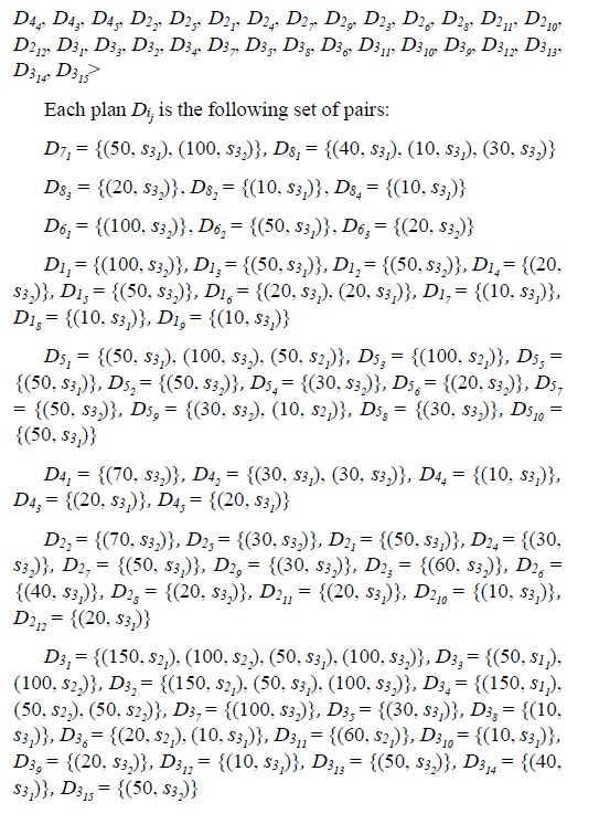
The processing plan is denoted as P = <D_ij, …, D_nk>, where D_ji is a set of plans for an operation e_i, where e_i is in E_sj. Each plan is a pair and is denoted as (B_i, s_ni) and B_i is the total number of input/output data blocks located in partition i in tier l_n (index of s_ni). If l_j = l₀, then the data blocks are located at the lowest tier in the multi-tiered storage.

After the output result of the operation e_i is allocated, unnecessary temporary input storage of operation e_i needs to be removed from multi-tiered persistent storage according to the persistent storage release plan. The persistent storage release plan is denoted as a sequence of pairs δ = < (e_i, (B_k, …, B_h)), …, (e_j, (B_x, …, B_y))>, where each pair (e_i, (B_k, …, B_h) is a group of data sets (B_k, …, B_h) that can be released after the results of an operation e_i are saved.

Then, the total processing time to read (B_i, s_ij) data blocks located at partition j in tier l_i is T_Bi = B_i * r_i. Formula (1) given below determines the total processing time T_r to read the data blocks for each input data set D_i = {(B₁, s_nj), …, (B_m, s_kn)}.

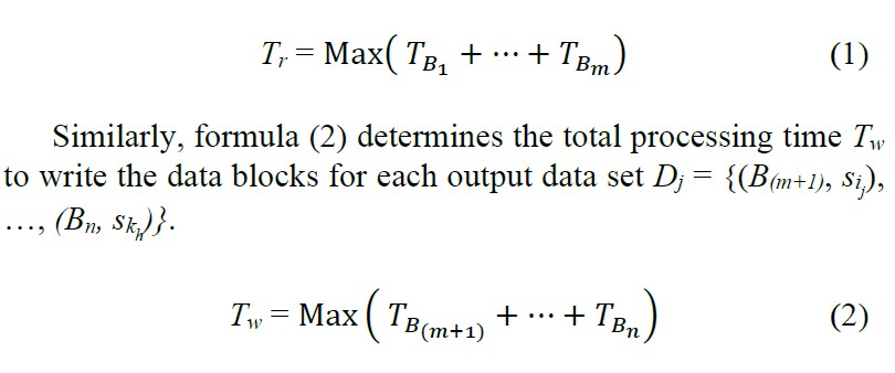
Let an Extended Petri Net <B, E, A, W> represent a query processing plan. Then, whenever it is possible, the output data sets of the operations E = {e_i, …, e_k} are written to the tiers located above the tiers of their input data sets. In other words, whenever possible, each operation tries to push up the results of its processing towards the partition at the higher tiers of persistent storage.

The benefits of such a strategy are as follows. First, it is faster to write the output data sets at a higher tier than at a lower tier. Second, the data sets written at a higher tier can be read faster by the next operation in a pipeline of a query processing plan. Therefore, the benefits include the time we gain from writing output data sets to the higher tiers and from reading the same data sets by the other operations.

3. Resource Allocation for a Single Query

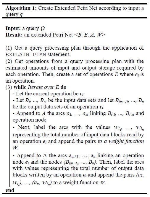
This section describes the algorithms that convert a query processing plan obtained from the execution of EXPLAIN PLAN statement for a single query into an Extended Petri Net and serialize the operations of the Net in order to minimize the amounts of persistent storage required for query processing.

3.1. Creation of Extended Petri Net

We consider a query Q expressed as a SELECT statement and submitted for processing by a relational database server operating on multi-tiered persistent storage. A query Q is ad-hoc processed by the system in the following way. First, a query optimizer transforms the query into the best query processing plan. SQL statement EXPLAIN PLAN can be used to list a plan found by a query optimizer. Next, the implementations of extended relational algebra operations such as selection, projection, join, anti-join, sorting, grouping, and aggregate functions are embedded into the query processing plan. Then, the plan is converted into an Extended Petri Net.

Operation e_j Î E where e_j is member of query Q. Each operation has the estimated amounts of input data to be read from persistent storage and the estimated output amounts of data to be saved in persistent storage. Algorithm 1 below transforms a query Q into an Extended Petri Net.

The algorithm obtains a query processing plan from the results of the EXPLAIN PLAN statement. From there, we get a set of operations E = {e_i, …, e_m}. A query processing plan provides information about the input data sets read by the operations and the output data sets written by the operations. The permanent and temporary data sets read and written by the operations in E form a set of places B in Extended Petri Net. The arcs leading from the input data sets to the operations and the arcs leading from the operations to the output data sets create a set of arcs A. A query processing plan provides information about the amounts of storage read and written by the operations. Such values contribute to the weight values w_j attached to each arc and are represented by a pair (a_j, w_j) in W. A weight value w_j attached to an arc between the input data set and an operation represents the total number of data blocks read by the operation. A weight value w_j attached to an arc between the operation and output data set represents the total number of data blocks written by the operation.

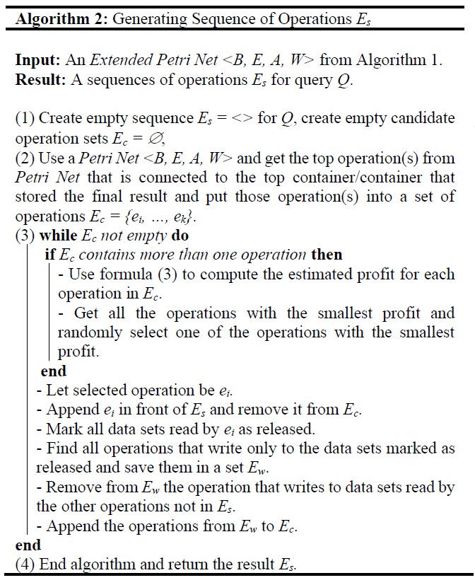
3.2. Serialization of Extended Petri Net

Preparation of an Extended Petri Net <B, E, A, W> for processing requires serialization of its operations in a set E. Serialization arranges a set of operations E into a sequence of operations E_s. There exist many ways that the operations in E can be serialized in the implementations of more complex queries. If the operations in E can be serialized in more than one way, then we try to find a serialization that requires smaller amounts of persistent storage for its processing. Algorithm 2 finds a serialization of operations in E that tries to minimize the total amounts of persistent storage allocated during query processing. As a simple example, consider an Extended Petri Net given in Figure 3. The operations e₁ and e₂ write 100 and 200 units of persistent storage. Then, 100 units of persistent storage are released after the processing of operations e₃ and e₆, and 200 units of persistent storage are released after the processing of operations e₃ and e₄. Since the processing of e₃ and e₄ releases more storage, we assign e₃ and e₄ before e₆ in the serialization.

A root operation in E is an operation such that at least one of its input arguments is a permanent data set that belongs to the contents of a database. A top persistent storage data set in B is a data set that contains the final results of query processing and such that is not read by any other operation in E. It is possible that a query may output more than one top persistent storage data set. A top operation is an operation that writes only to the top persistent storage data sets.

Algorithm 2 traverses the arrows in A backward from the top operations to the root operations and generates a sequence of operations E_s from a set of operations E.

At the very beginning, a sequence of operations E_s is empty, and none of the persistent storage data sets in B is marked as released. In the first step, the algorithm finds the top operations and inserts such operations into a set of candidate operations E_c.

For each operation in E_c, the algorithm computes profit using formula (4). To compute profit, the algorithm deducts the total amounts of persistent storage allocated by an operation from the total amounts of persistent storage released by an operation. For example, assume that the current operation is e_i. To find the amounts of persistent storage released by an operation e_i, we perform the summation of the amounts of storage in all input data sets of operation e_i not marked as released yet. It is denoted by . To find the profits from the processing of an operation e_i, we deduct from the released amounts the amounts of persistent storage included in the output data sets of the operation and denoted as  in formula (3) below.

The profits are computed for each operation in E_c. The algorithm selects an operation with the smallest profit. If more than one operation has the smallest profit, then the algorithm randomly chooses one of them. Let a selected operation be e_i. The algorithm removes e_i from E_c, appends it in front of E_s, and marks all data sets read by e_i as released. Next, the algorithm finds the operations that write only to data sets marked as released by e_i, such that data sets released by e_i are read only by the operation already in E_s. An objective is to find the operations that can be appended to E_c in a correct order of processing determined by a set of arcs A. Then, the algorithm appends those selected operations to a set of candidate operations E_c and the profits for each operation in E_c are computed again. An operation with the lowest profits is appended in front of E_c. The algorithm repeats the procedure until all operations in E are appended in front of E_s.

Example1: The example explains a sample trace of Algorithm 2 when applied to an Extended Petri Net given in Figure3. In the first step, E_c contains only one operation e₈ connected to top data set B₁₁. Therefore, e₈ has the lowest profit in E_c. We append it in front of E_s = <e₈> and we remove it from E_c. The data sets B₅, B₆, and B₇ read only by e₈ are marked as released. The operations writing only to the data sets B₈, B₉, and B₁₀ are e₅, e₆, e₇. None of the data sets B₈, B₉, and B₁₀ are read by an operation that is not in E_s. Hence the operations e₅, e₆, e₇ can be added to E_c = {e₅, e₆, e₇}. The estimated profits for each operation computed with a formula (3) are the following: p(e₅) = (0 – 400) = -400, p(e₆) = (100 – 50) = 50 and p(e₇) = (430 – 300) = 70. According to those results, e₅ is picked, appended in front of E_s = <e₅, e₈>, and removed from E_c = {e₆, e₇}. A data set B₇ is an input data set, and it cannot be marked as released. As no new data sets are released, E_c remains the same. Next, an operation e₆ which has the second smallest profit, is taken from E_c. It is appended in front of E_s = <e₆, e₅, e₈> and is removed from E_c = {e₇}. A data set B₃ read by e₆ is marked as released. A data set B₃ is marked as written by operation e₁ and later it is read by e_3. In this case, e₁ cannot be appended to E_c because a data set B₃ is read by e₃ that is not assigned to E_s yet. Next, e₇ is taken from E_c, it is appended in front of E_s = <e₇, e₆, e₅, e₈>, and is removed from E_c. A data set B₅ read by e₇ is marked as released. A data set B₅ is written by the operations e₃ and e₄. Both operations are appended to E_c = {e₃, e₄}. The computations of the profits provide: p(e₃) = 0 – 280 = -280 and p(e₄) = 0 – 150 = -150. According to the results, e₃ is appended in front of E_s = <e₃, e₇, e₆, e₅, e₈> and it is removed from E_c = {e₄}. The data sets B₃ and B₄ read by e₃ are marked as released. The operations e₁ and e₂ are written to data sets B₃ and B₄. An operation e₁ can be appended into E_c because e₆ that read B₃ is already assigned in E_s. An operation e₂ cannot be appended into E_c = {e₁, e₄} because e₄ that reads a data set B₄ is not in E_s yet. The computations of the profits provide: p(e₁) = 0 – 100 = -100 and p(e₄) = 200 – 150 = 50. According to the results, e₁ is appended in front of E_s = <e₁, e₃, e₇, e₆, e₅, e₈> and is removed from E_c = {e₄}. Operation e₁ reads an input data set, therefore, no new operations can be added to E_c. Next, operation e₄ is append to E_s = <e₄, e₁, e₃, e₇, e₆, e₅, e₈> and is removed from E_c. A data set B₄ read by e₄ is marked as released and operation e₂ is appended to E_c. Finally, operation e₂ is appended in front of E_s = <e₂, e₄, e₁, e₃, e₇, e₆, e₅, e₈>. Operation e₂ reads from an input data set and because of that, no more operations can be assigned to E_c. The final sequence of operations E_s = <e₂, e₄, e₁, e₃, e₇, e₆, e₅, e₈> is generated at the end.

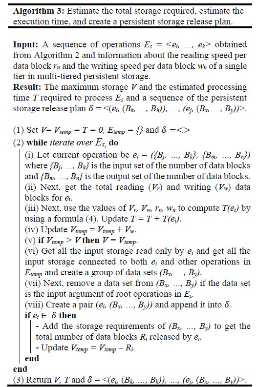
3.3  Estimation of Storage Requirements and Generation of Persistent Storage Release Plan

A sequence of operation E_s obtained from the linearization of an Extended Petri Net with Algorithm 2 is used to estimate the requirements on the amounts of persistent storage needed for the processing of the sequence. Algorithm 3 estimates the persistent storage requirements while processing the operations in E_s. The output of Algorithm 3 is the estimated processing time T for E_s using the read/write speed of single-tier, the maximum required storage V to process E_s, and a sequence of the persistent storage release plans  = <(e_i, (B_k, …, B_h)), …, (e_j, (B_x, …, B_y))>.

      Algorithm 3 uses a sequence of operations E_s and information about reading speed per data block r_n and writing speed per data block w_n parameters unchanged and extracted from a single tier in multi-tiered persistent storage. Typically, the algorithm is processed with the read/write parameters of the highest tier. First, the algorithm sets V = 0, which stores the maximum storage required to be allocated in the multi-tiered persistent storage, and T = 0, which stores the estimated processing time for E_s. Next, the algorithm iterates over E_s in step (2) in Algorithm 3 and lets the current operation be e_i. First, the total read storage V_r is computed by summing all input storage for e_i and the total write storage V_w is computed by summing all output storage for e_i. After that, the current temporary storage V_temp = V_temp + V_w is updated, where V_temp stores the temporary storage required to process until the current operation. Next, the algorithm compares V_temp with V. If V_temp is larger than V, then V = V_temp is updated. Next, the algorithm computes the estimated total processing time t_i for current operation e_i using the following equation.

      T(e_i) = (V_r * r_n) + (V_w * w_n)                                       (4)

Then, the algorithm updates the total processing time until operation e_i by summing T = T + T(e_i).

Next, the algorithm gets the storage released by operation e_i, denoted as a pair (e_i, (B_x, …, B_y)). The detailed procedure is shown from step (2)(vi) to step (2)(viii) in the algorithm. After this, the storage is appended into the persistent storage release plan .

If e_i is the member of  then the algorithm needs to release data blocks after the output data blocks of e_i are allocated. Next, the algorithm needs to update V_temp = V_temp – the total number of release storage by e_i.

Algorithm 3 iterates those procedures above for each operation from the input sequence E_si. Finally, Algorithm 3 will generate V, T, and  = <(e_i, (B_k, …, B_h)), …, (e_j, (B_x, …, B_y))>.

Example 2: A sample trace of Algorithm 3 is performed on a sequence of operations E_s = <e₂, e₄, e₁, e₃, e₇, e₆, e₅, e₈> from Example 1 together with the reading and writing speed per data block from the highest tier l₃ = (0.05, 0.055, <500, 300, 100>). As it has been mentioned before, the reading and writing speed per data block is measured in the standardized time units.

         At the very beginning, we set V = V_temp = T = 0, and . Next, we iterate over E_s, and let the current operation be e₂. It reads V_r = 300 data blocks and writes V_w = 200 data blocks. Next, we compute t₂ = (300*0.05) + (200*0.055) = 26 and update T = T + t₂ = 26. Then, we set V_temp = V = 200. A persistent storage release plan  remains empty because e₂ is the first operation in the sequence E_s.

In the next iteration, the current operation is e₄. We compute t₄ = (200*0.05) + (150*0.055) = 18.25 and update T = 26 + 18.25 = 44.25 and V_temp = 200 + 150 = 350. Due to V_temp being larger than V, we increase V = 350. The operation does not release storage and there is no need to update

In the next iteration e₁ is the current operation.  T  = 59.75, V_temp = 350 + 100 = 450 and V= 450.

 In the next iteration e₃ is the current operation.  T = 90.15, V_temp = 450 + 280 =730 and V = 730. This time, e₃ released 200 data blocks, therefore, we need to update  = <(e₃, (B₄))>. Total number of data blocks released by e₃ is 200. Therefore, we update V_temp = 730 – 200 = 530.

In the next iteration, e₇ is the current operation.  T = 128.15 and V_temp = 530 + 300 = 830 and V= 830. This time we release storage B₅ and update  = <(e₃, (B₄)), (e₇, (B₅)) > and V_temp = 830 – 430 = 400.

In the next iteration, e₆ is the current operation.  T = 135.9 and V_temp = 400 + 50 = 450 and V= 830. The storage released by e₆ is B₃ and update  = <(e₃, (B₄)), (e₇, (B₅)), (e₆, (B₃)) > and V_temp = 450 – 100 = 350.

In the next iteration, e₅ is the current operation. The algorithm computes T = 182.9 and V_temp = 350 + 400 = 750 and V= 830. An operation e₅ does not release any storage.

The last operation from the sequence E_s is e₈. The algorithm computes T = 247.9 and V_temp = 750 + 500 = 1250 and V= 1250. This operation releases three storages, B₈, B₉, and B₁₀. The updated storage released plan is  = <(e₃, (B₄)), (e₇, (B₅)), (e₆, (B₃)), (e₈, (B₇, B₈, B₉))>.

Finally, Algorithm 3 returns T = 247.9 of time units, V = 1250 data blocks and  = <(e₃, (B_i4)), (e₇, (B₅)), (e₆, (B₃)), (e₈, (B₇, B₈, B₉))> for a sequence of operations E_s.

4. Resource Allocation for a Group of Queries

Algorithm 4 takes on input a set of query processing plans {E_s1, …, E_sn} created by Algorithm 2, a set of estimated processing times  = {T₁, …, T_n}, a set of maximum storage requirements for each processing plan  = {V₁, …, V_n}, a set of deallocation plans  from the Algorithm 3, and a sequence of persistent storage tiers L = <l₀, …, l_n>. The output of the algorithm is a sequence of storage allocation plans P.

First, the algorithm gets the estimated processing time T and the estimated highest allocation storage V for processing plans from . Next, the algorithm collects the candidate operations from , where a candidate operation is the first operation from each sequence, and puts them into a set of candidate operations E_c. Next, the algorithm picks one operation from E_c in the following way. First, the algorithm picks the operations from the sequences with the smallest volume, V. If more than one operation is found, then from the operations found so far, the algorithm picks the operations from the sequences with the shortest time, T. If again more than one operation is found, then the algorithm uses formula (3) to compute a profit for each operation and picks the operations with the highest profit. Again, if more than one operation is still found, then the algorithm randomly picks one operation. Let selected in this way, the candidate operation be e_i = ({B_i, …, B_j}, {B_k, …, B_h}), and the total number of data blocks in output data sets of the operation be V_w.

Algorithm 4 passes the information about L, V_w, and P to Algorithm 4.1 to find the best partition and generate the updated storage allocation plan P. Next, Algorithm 4 must update L with information about temporary storage to be released after the processing of e_i. To do so, Algorithm 4 passes a deallocation plan  for E_si, a sequence of tiers L, and the operation e_i to Algorithm 4.2 to update information about available storage in L.

Finally, an operation e_i is removed from E_si. The algorithm repeats the steps above for each operation from each sequence until all sequences are empty. The algorithm returns the final storage allocation plan P.

Algorithm 4: Generating storage allocation plans
Input: A set of processing plans  {Es1, …, Esn} from algorithm 2, deallocation plan , the maximum storage V, and the estimated processing time T for each sequence from Algorithm 3. A sequence of tiers L = <l0, …, ln> where each tier li is described as triple (ri, wi, <sij, …, sii>). Result: A sequence of allocation plans P = <Dij, …, Dnk>.
(1) Create empty sequence of allocation plans P = < >. (2) While until all sequences in  are empty do
	– Create an empty set of candidate operations Ec = {}. – Get the first operations from the sequences with the smallest volume V and put them into Ec.
	if more than one operation is found in Ec then
		– Keep the operations from the sequence Es1, …, Esn with the smallest estimated processing time T and remove the rest of the operations from Ec.
	else if more than one operation is found in Ec then
		– Keep the operations with the highest profit using formula (3) and remove the rest of the operations from Ec.
	else if more than one operation is found in Ec then
		– Select one operation randomly and make Ec empty.
	end – Let the selected operation be ei = {Bi, …, Bj}, {Bk, …, Bh} from Esj and its input storage be {Bi, …, Bj} and its output storage be {Bk, …, Bh}. – Let the number of total output storage be Vw. – Use the information of L, Vw, and P to find the best partition using Algorithm 4.1 and get the result of updated plan P from algorithm 4.1. – Pass the information about a deallocation plan , a state of multi-tiered persistent storage L, and the operation ei to Algorithm 4.2 to update L with information about temporary storage released by ei. – Remove ei from Esj. – Update estimated processing time T and V for Esj.
end
(3) Return the sequence of multi-tiered storage allocation plans P = <Dij, …, Dnk>.

Algorithm 4.1 finds the best partition using the information in L, V_w, P and e_i provided by Algorithm 4.

Let e_i be a member of E_sj, and a set of allocation plans for e_i is denoted D_ji. First, the algorithm needs to find the best partition located at the highest possible tier in order to achieve the best processing time. Next, the algorithm finds a partition that can accommodate the storage V_w where V_w is the total output storage required to store the temporary/permanent result of e_i. The input storage {B_i, …, B_j} is already assigned to one of the partitions on L. Therefore, the algorithm needs to find the best storage allocation for V_w only.

Next, the algorithm iterates over the tiers in L. Let the current tier be (r_n, w_n, <s_nj, …, s_ni>). The algorithm needs to check whether the required storage V_w can be allocated entirely in one partition or over more partitions. When the amount of storage available at one of the partitions in the highest tier is larger or equal to V_w, the algorithm creates an allocation plan (B_i, s_nj) where B_i = V_w and appends that plan to D_ji. But sometimes, the amounts of storage available at all partitions in the highest tier are smaller than the required storage V_w. In that case, the algorithm splits storage V_w into multiple storages V_w‘, …, V_w”. Some storage is to be allocated at the faster tier, and some may be at the lower tier. For that case, the algorithm splits V_w to allocate more than one partition and creates allocation plans (B_i, s_nj), …, (B_j, s_nk). Next, the algorithm appends all those plans into D_ji. Finally, the allocation plan D_ji is appended to P and returned to Algorithm 4.

Algorithm 4.1: Finding the best partition and generating a plan for storage allocations
Input: A multi-tiered persistent storage L = <l0, …, ln>, storage requirements Vw of an operation ei, a sequence of storage allocation plans P. Result: The updated sequence of storage allocation plans P.
(1) Let the amounts of temporary storage Vtemp = 0 and let an initial storage allocation plan Dji for the operation ei be empty.
(2) while iterate over L in reverse order do
	(i) Let current tier be li = (ri, wi, <sii, …, sin>) and let <sii, …, sin> be a sequence of partitions in li arranged from the smallest to the largest partition. (ii) Iterate over partitions <sii, …, sin> and choose a partition sik such that its size is equal or larger than Vw.
	(iii) if size of sik is larger or equal to Vw then
		– Create a pair (Bi, sni) where Bi = Vw and append it into Dji. – Update sik = sik – Vw and Vw = Vtemp. – Sort a sequence of partitions arranged from smallest available storage to largest available storage.
	else if all storage in current set is smaller than Vw then
		– Update Vtemp = Vw. while iterate over partition in reverse order and until Vtemp = 0 or all available storage become zero do
			– Let the current storage in a set be sik. – Split storage into two parts: Vw, where Vtemp = Vtemp – sni and Vw = sik – Create a pair (Bi, sik) where Bi = Vw and append it into Dji. – Update sii = 0, and Vw = Vtemp. – Sort a sequence of partitions arranged from smallest available storage to largest available storage.
		end
	end
end (3) Append Dji = {(Bi, sni), …, (Bj, smk)} into P.
(4) Return P.

Algorithm 4.2 releases persistent storage no longer needed by an operation e_i. An input to the algorithm is a deallocation plan , a sequence of tier L = <(r_n, w_i, <s_ni, …, s_ni>), …, (r₀, w₀, <s_n0, …, s_nj>)>, and the operation e_i passed from Algorithm 4.

Algorithm 4.2 checks whether e_i releases any persistent storage. If e_i is a member of the deallocation plan , then the algorithm needs to update L according to the deallocation plan, such as removing the storage released by e_i from the occupied storage_. If e_i is not a member of the deallocation plan, then the algorithm does not need to update L.

Algorithm 4.2: Deallocation the storage
Input: A deallocation plan , a multi-tiered persistent storage L = <l0, …, ln>, and the operation ei. Result: The updated multi-tiered persistent storage L = <l0, …, ln>.
(1) if ei  then
	– Get the storage released by ei like (Bx, …, By).
	while iterate over (Bx, …, By) do
		– Let current storage be Bi and the location of Bi be (Bi, shi) where storage Bi is located at partition i from tier lh. – Remove a storage Bi from partition i in level lh and update shi = shi + Bi. – Let shi is belong to the sequence <shx, …, shy>. – Sort a sequence of partitions <shx, …, shy> arranged from smallest available storage to largest available storage.
	end
end
(2) Return the updated L = <l0, …, ln>.

      Algorithm 5 computes the total processing time T_f for the allocation plan P created by Algorithm 4. First, the algorithm iterates over plan P. Let the current set of plans be D_ji = {(B_i, s_ni), …, (B_j, s_ik)} where D_ji is a set of plans for the operation e_i in sequence E_sj. Next, the algorithm iterates over D_ji. Let the current pair be (B_i, s_ni). Then, the algorithm computes the processing time for that pair. If B_i is a member of input data blocks for e_i, then compute T_f = T_f + (B_i * r_n) where r_n is a reading speed per data block. If B_i is the member of output data blocks for e_i, then compute T_f = T_f + (B_i * w_n) where w_n is a writing speed per data block. Next, the algorithm checks whether e_i is the last operation in the sequence E_sj or not. If e_i is the last operation, then the algorithm needs to compute the reading time for final storage such as T_f = T_f + (V_w * r_n), where V_w is the total data blocks written by operation e_i. Finally, the algorithm returns the total execution time for plan P.

Algorithm 5: Final estimated processing time for allocation plan
Input: A sequence of allocation plans P = <Dij, …, Dnk>. Result: Total estimated processing time Tf for allocation plan P.
(1) Let total processing time for sequences be Tf = 0. (2) while iterate over P do
	– Set total writing data block be Vw = 0. – Let the current plan be Dji = {(Bi, sni), …, (Bj, sik)} for operation ei = {Bi, …, Bj}, {Bk, …, Bh} from Esj.
	while iterate over Dji then
		– Let current pair be (Bi, sni) where Bi is a total number of data blocks allocated at a tier n in a partition i (sni). if Bi is member of input storage {Bi, …, Bj} then
			– Tf = Tf + (Bi * rn)
		else
			– Tf = Tf + (Bi * wn)
		end
	end
	if ei is the last operation from Esj then
		– Read the final result and release the storage. – Update Tf = Tf + (Vw * rn).
	end
end
(3) Return total processing time for allocation plan Tf.

Example 3: In this example, we use a multi-tiered persistent storage with 3 tiers. We assume that the highest tier l₂ has 3 partitions, the lower one l₁ has 2 partitions, and the bottom tier l₀ has 3 partitions. The parameters of the tiers are listed below.

L = <l₀, l₁, l₂>

• l₀ = (0.2, 0.21, <200, 500, 1000>)
• l₁ = (0.1, 0.105, <100, 200>)
• l₂ = (0.05, 0.055, <40, 50>)

Next, we use a set of sequences  {E_s1, E_s2, E_s3}. A sequence E_s1 consists of the following 3 operations E_s1 = <e₁, e₂, e₃> where

• e₁ = ({50, 50}, {100})
• e₂ = ({100}, {50})
• e₃ = ({50}, {20})

The total estimated processing time for E_s1 is T₂ = 37.85 and V₁ = 150.

The sequence E_s2 consists of one operation, E_s2 = < e₁> where

• e₁ = ({150}, {100})

The total estimated processing time for E_s2 is T₂ = 40.50 and V₂ = 100.

The last sequence E_s3 consists of 4 operations E_s3 = < e₁, e_3, e_2, e_4, > where

• e₁ = ({50}, {40, 40})
• e₂ = ({40}, {20})
• e₃ = ({40}, {10})
• e₄ = ({30}, {10})

The total estimated processing time for E_s3 is T₃ = 22.60 and V₃ = 110.

Following step (2) of Algorithm 4, we picked an operation e₁ from sequence E_s2, because V₂ is the smallest volume, and put it into E_c = {e₁}. Since we have only one candidate operation, it is passed to Algorithm 4.1 to find the storage allocations for the outputs of operation e₁. According to Algorithm 4.1, the best storage is s₂₃ and therefore, we created a plan like (100, s₂₃). We then appended the plan into P = <(100, s₂₃)>. Next, Algorithm 4 released storage if e₁ needs to release some storage. According to Algorithm 4.2, e₁ does not need to release any storage. We repeated the above procedure and finally get the plan P for  where P = <{(40, s₂₁), (50, s₂₂), (10, s₁₁)}, {(40, s₂₁), (40, s₂₂)}, {(10, s₂₂), (10, s₁₁)}, {(10, s₂₁)}, {(10, s₂₁)}, {(40, s₂₁), (50, s₂₂), (10, s₁₁)}, {(50, s₁₁)}, {(20, s₂₁)}>.

Next, we compute the processing time for a sequence of plan P by using the algorithm 5. The total processing time T_f for  is 112.55 time units. With random allocation, the total processing time for  become 143.45 time units. Without multi-tiered persistent storage with partitions, the total execution time for  is 219.90 time units.

5.      Example/Experiment

Different types of persistent storage devices such as SSD, HDD, and NVMe can be used to create a multi-tiered persistent storage system. In the experiment, we picked a sample multi-tiered persistent storage L that consists of 4 tiers <l₀, l₁, l₂, l₃>, where l₃ is the fastest tier such as NVMe and l₀ is the slowest tier, such as HDD and l₂ and l₁ are faster and slower SSDs. Each tier is divided into two partitions of different sizes. Table 1 shows the read and write speed per data block expressed in standardized time units and the total number of data blocks available at each partition.

Table 1: Read/Write Speed with Available Size for Multi-tiered Storage Devices

Level of Devices	Reading Speed	Writing Speed	Partition 1	Partition 2
l0	0.15 * 1­­03	0.155 * 1­­03	1000	2000
l1	0.1 * 1­­03	0.105 * 1­­03	500	600
l2	0.08 * 1­­03	0.085 * 1­­03	150	200
l3	0.05 * 1­­03	0.055 * 1­­03	50	100

In the experiment, we applied Algorithm 1 to convert eight query processing plans into the Extended Petri Nets. Next, we used Algorithm 2 to find the optimal sequences of operations for each Petri Net. Next, Algorithm 3 was used to get the deallocation plans , the maximum volumes V, and the estimated execution times T required for each sequence of operations found by Algorithm 2. The values for each sequence are the following.

E_s1= <e₁, e₃, e₂, e₄, e₅, e₆, e₇, e₈, e₉>

V₁ = 150, T₁ = 110.70

Table 2: Operations With Input and Output Data sets For E_s1

Operation	Input data set	Output data set
e1	300	100
e2	200	50
e3	100	50
e4	50	20
e5	50, 20	50
e6	50	20, 20
e7	20	10
e8	20	10
e9	10, 10	10

E_s2= <e₂, e₅, e₁, e₄, e₇, e₉, e₃, e₆, e₈, e₁₁, e₁₀, e₁₂>

V₂ = 300, T₂ = 108.35

Table 3: Operations with Input and Output Data sets For E_s2

Operation	Input data set	Output data set
e1	100	50
e2	100	70
e3	100	60
e4	50	30
e5	70	30
e6	60	40
e7	30, 30	50
e8	40	20
e9	50	30
e10	20	10
e11	30	20
e12	20, 10	20

E_s3= <e₁, e₃, e₂, e₄, e₇, e₅, e₈, e₆, e₁₁, e₁₀, e₉, e₁₂, e₁₃, e₁₄, e₁₅>

V₃ = 300, T₃ = 147.40

Table 4: Operations with Input and Output Data sets For E_s3

Operation	Input data set	Output data set
e1	500	400
e2	600	300
e3	400	100, 50
e4	300	200, 50
e5	100	30
e6	50	30
e7	200	100
e8	50	10
e9	30	20
e10	30	10
e11	100, 10	60
e12	20	10
e13	60	50
e14	50	40
e15	10, 10, 40	50

E_s4= <e₁, e₂, e₄, e₃, e₅ >

V₄ = 250, T₄ = 100.70

Table 5: Operations with Input and Output Data sets For E_s4

Operation	Input data set	Output data set
e1	80	70
e2	70	30, 30
e3	30	20
e4	30	10
e5	20, 10	20

E_s5= <e₁, e₃, e₅, e₂, e₄, e₆, e₇, e₉, e₈, e₁₀ >

V₅ = 200, T₅ = 93.50

Table 6: Operations with Input and Output Data sets For E_s5

Operation	Input data set	Output data set
e1	300	100
e2	100	50
e3	200	100
e4	50	30
e5	100	50
e6	30	20
e7	100	50
e8	50	30
e9	20, 50	40
e10	30, 40	50

E_s6 = <e₁, e₂, e₃>

V₆ = 150,        T₆ = 37.85

Table 7: Operations with Input and Output Data sets For E_s6

Operation	Input data set	Output data set
e1	50, 50	100
e2	100	50
e3	50	20

E_s7 = < e₁>

V₇ = 100, T₇ = 40.50

Table 8: Operations with Input and Output Data sets For E_s7

Operation	Input data set	Output data set
e1	150	100

      E_s8 = < e₁, e_3, e_2, e_4, >

V₈ = 110, T₈ = 22.60

Table 9: Operations with Input and Output Data sets For E_s8

Operation	Input data set	Output data set
e1	50	40, 40
e2	40	20
e3	40	10
e4	20, 10	10

Next, we used Algorithm 4 to decide on an order of concurrent processing of operations from the sequences in . Algorithms 4.1 and 4.2 were used within Algorithm 4 to find the best allocation of partitions and to generate a persistent storage allocation plan. The details of the plan are listed in the Appendix. After that, we used Algorithm 5 to simulate the processing of the plan to get the total estimated execution time T_f, see Table X.

In the second experiment, we used the same set of sequences of operations , and whenever more than one operation could be selected for processing, we randomly picked an operation. The total execution time for the second experiment is given in Table X.

In the third experiment, we used only a single tier of persistent storage, and like before, whenever more than one operation could be selected for processing, we randomly picked an operation. The final results of all experiments are summarized in a Table X.

Table 10: Summary of Experimental Results

Experiment	Method	Total execution time-units
Experiment 1	Using allocation plan over multi-tiered persistend storage that proposed in this work.	857
Experiment 2	Using random allocation plan over multi-tiered persistend storage.	1,068.35
Experiment 3	Using allocation plan without multi-tiered persistend storage.	1,466.95

By comparing those three results, one can find that the execution plan for experiment 1 achieves better performance and faster execution time than experiment 2 and experiment 3.

6.      Summary and Future Work

This paper presents the algorithms that optimize the allocations of persistent storage over a multi-tiered persistent storage device when concurrently processing a number of database queries. The first algorithm converts a single query processing plan obtained from a database system into an Extended Petri Net. An Extended Petri Net represents many different sequences of database operations that can be used for the implementation of a query processing plan. The second algorithm finds in an Extended Petri Net a sequence of operations that optimizes storage allocation in multi-tiered persistent storage when a query is processed. The third algorithm estimates the maximum amount of persistent storage and processing time needed when a sequence of operations found by Algorithm 2 is processed.

In the second part of the paper, we considered the optimal allocation of multi-tiered persistent storage when concurrently processing a set of queries. We assumed that the first three algorithms are used for individual optimization of storage allocation plans for each query in a set. The fourth algorithm optimizes the allocation of multi-tiered persistent storage when a set of sequences of operations obtained from the first three algorithms is concurrently processed. The algorithm creates a persistent storage allocation and releases a plan according to the available size and speed of the devices implementing multi-tiered persistent storage.

The last algorithm processes a storage allocation plan created by the previous algorithm and returns the estimated processing time. To validate the proposed algorithms, we conducted several experiments that compared the efficiency of processing plans created by the algorithms with the random execution plans and execution plans without multi-tiered persistent storage. According to the outcomes of experiments, the storage allocation plans obtained from our algorithms consistently achieved better processing time than the other allocation plans.

Several interesting problems remain to be solved. An optimal allocation of persistent storage in the partitions of multi-tiered storage contributes to a dilemma of spreading a large allocation over smaller allocations at many higher-level partitions versus a single allocation at a lower partition.

Another interesting question is related to a correct choice of a level at which storage is allocated depending on the stage of query processing. It is almost always such that the initial stages of query processing operate on the large amounts of storage later reduced to the smaller results. It indicates that the early stages of query processing should be prioritized through storage allocations at higher levels of multi-tiered storage. It means that the parameters of multi-tiered storage allocation may depend on the phases of query processing with faster storage available at early stages.

The next interesting problem are the alternative multi-tiered storage allocation strategies. In one of the alternative approaches, after the serialization of Extended Petri Nets representing individual queries, it is possible to combine the sequence of operations into one large Extended Petri Net and apply serialization again. Yet another idea is to combine the Extended Petri Nets of individual queries into one Net and try to eliminate multiple accesses to common data containers.

The next stimulating problem is what to do when the predictions on the amounts of data read and/or written to multi-tiered persistent storage do not match the reality. A solution for these cases may require ad-hoc resource allocations and dynamic modifications of existing plans.

It is also possible that a set of queries can be dynamically changed during the processing. For example, a database application can be aborted, or it can fail. Then, the management of persistent storage also needs to be dynamically changed. A solution to such a problem would require the generation of a plan with the options where certain tasks are likely to increase or decrease their processing time.

Conflict of Interest

The authors declare no conflict of interest.

Acknowledgment

I would also like to extend my thanks to the anonymous reviewers for their valuable time and feedback. Finally, I wish to thank my parents for their support and encouragement throughout my study.

1. Data Storage Trends in 2020 and Beyond, https://www.spiceworks.com/marketing/reports/storage-trends-in-2020-and-beyond/ (accessed on 30 April 2021)
2. U. Sivarajah, M. M. Kamal, Z. Irani, V. Weerakkody, “Critical Analysis of Big Data Challenges and Analytical methods”. In Journal of Business Research, vol. 70, pp. 263–286, 2017.
3. S. wang, Z. Lu, Q. Cao, H. Jiang, J. Yao, Y. Dong, P. Yang, C. Xie, “Exploration and Exploitation for Buffer-controlled HDD-Writes for SSD-HDD Hybrid Storage Server”, ACM Trans. Storage 18, 1, Article 6, February 2022.
4. Apache Ignite Multi-tier Storage, https://ignite.apache.org/arch/multi-tier-storage.html (accessed on 30 April 2021)Trans. Roy. Soc. London, vol. A247, pp. 529–551, April 1955.
5. Tiered Storage, https://searchstorage.techtarget.com/definition/tiered-storage (accessed on 30 April, 2021).
6. E. Tyler, B. Pranav, W. Avani, Z. Erez, “Desperately Seeking Optimal Multi-Tier Cach Configurations”, In 12th USENIX Workshop on Hot Topics in Storage and File System (HotStorage 20), 2020.
7. H. Shi, R. V. Arumugam, C. H. Foh, K. K. Khaing, “Optimal disk storage allocation for multi-tier storage system”, Digest APMRC, Singapore, 2012, pp. 1-7.
8. N.N. Noon, “Automated performance tuning of database systems”, Master of Philosophy in Computer Science thesis, School of Computer Science and Software Engineering, University of Wollongong, 2017.
9. N.N. Noon, J.R. Getta, “Optimisation of query processing with multilevel storage”, Lecture Notes in Computer Science, 9622 691-700. Da Nang, Vietnam Proceedings of the 8th Asian Conference, ACIIDS 2016.
10. B. Raza, A. Sher, S. Afzal, A. Malik, A. Anjum, Adeel, Y. Jaya Kumar, “Autonomic workload performance tuning in large-scale data repositories”, Knowledge and Information Systems. 61. 10.1007/s10115-018-1272-0.
11. N.N. Noon, J.R. Getta, T. Xia, “Optimization Query Processing for Multi-tiered Persistent Storage”, IEEE 4th International Conference on Computer and Communication Engineering Technology (CCET), 2021, pp. 131-135, doi: 10.1109/CCET52649.2021.9544285.
12. R. Wolfgang, “Understanding Petri Nets: Modeling Techniques, Analysis Methods, Case Studies”, Springer Publishing Company, Incorporated, 2013.

(Click Here)