1. Introduction

City planning initiatives can benefit from insights into mobility patterns of pedestrians and vehicles. Given the prevalence of WiFi- enabled devices carried by individuals and their continuous emission of WiFi probe requests, such mobility patterns can be revealed by localization of the devices based on measurements of WiFi probe requests via the recorded received signal strength indicator (RSSI). Active and passive localization are the two standard modes of RSSI- based localization [1]. Active localization occurs on the target device with the help of a custom app that may or may not require cooperation (e.g., data exchange); it answers the question “Where am I?” Passive localization occurs without the device’s knowledge in an anonymous manner; it answers the question “Where are you?” Due to the apparent difficulty of large-scale mobile app adoption for localization purposes, passive localization is the more realistic choice.

High variability in RSSI measurements due to fading (path-loss), shadowing (temporary obstruction between a sender and a receiver), and interference (overlap of WiFi channels) is a significant challenge in RSSI-based localization [2]. To mitigate RSSI variability, some active localization methods leverage device cooperation to obtain additional location-sensitive information, such as signal angle of arrival [3, 4], round-trip time [5], device orientation [6], and device prior location [7]. However, passive localization cannot benefit from

device cooperation [8]–[13]. Since the operations of these methods

share similarities with passive localization, they might be transfer- able. However, fundamental differences exist between the two. For instance, missing data are unlikely in active localization because the probing signal is emitted by the access points in large numbers. In passive localization, the probing signal is initiated by the target device in an uncontrolled and sporadic manner. Consequently, the active localization methods may have data requirements unachievable in passive localization.

Previous work has also explored methods tailored to passive localization. However, they typically suit applications on a very small (indoor) or very large scale (entire city), making them inadequate for applications on a medium scale (within the span of a city street) (see Section 2.2 for details).

Therefore, investigation into methods suitable for RSSI-based passive localization in urban areas at the scale of a city street is necessary. The investigation can be divided into two parts. One focuses on the feasibility of adapting the methods used in cooperation-free active localization (hereinafter referred to as “traditional active localization methods”) to passive localization; the other focuses on new approaches not fully explored by previous research on passive localization.

To facilitate the investigation, we have developed a privacy centric mobility intelligence system (MobIntel) consisting of sensors and cloud infrastructure to collect and analyze RSSI measurements from anonymized WiFi probe requests. MobIntel has been tested in downtown West Palm Beach, Florida, to count the number of WiFi-enabled devices in a sensor’s visible range and to calculate the percentage of devices that have persisted over time [14].

In this paper, which is an extension of the work initially presented in WiMob 2021 [15], we discuss a significant augmentation to the analytical facilities of MobIntel, exploring methods to conduct passive localization in a controlled environment, with the goal of identifying methods that are performant at the scale of a city street (1.4 km). The specific contributions of the paper include:

1. We conduct a systematic performance evaluation of two adaptations of traditional active localization methods—path-loss- based multilateration and fingerprinting—to support passive localization. We examine performance impacts under vary- ing training and testing data sets, including (1) training and testing on individual RSSI measurements, (2) training and testing on averaged RSSI measurements, and (3) training on averaged, but testing on individual RSSI measurements. We also compare the performance of fingerprinting across three implementation methods, including vector-based Eu- clidean distance, Gaussian-based area-under-the-curve, and Gaussian-based tail
2. For Gaussian-based fingerprinting in particular, we discover that the previously reported area-under-the-curve method, based on the arithmetic mean of the area-under-the-curve in a Gaussian distribution [7], does not perform well when there is large mismatch between the unknown RSSI measurements and the fingerprint of a reference point. We propose an alternative method, which uses the Gaussian tail probability as the likelihood of the unknown RSSI measurements originating from a particular reference We show that our proposed method achieves better localization performance.
3. We carry out a systematic evaluation of the accuracy impact of integrating machine learning algorithms—multi-layer perceptron, support vector machine, and K-nearest neighbors—with traditional active localization methods. We demonstrate that the machine learning-based methods outperform their traditional counterparts, regardless of which model is incorporated, or which training or testing set is

This paper is organized as follows. Section 2 provides a brief overview of related work in RSSI-based active and passive localization. Section 3 describes how we adapt the localization method from a traditional active context to a passive context and how we incorporate machine learning methods to boost performance. Section 4 presents details of data collection, including experimental design, hardware configuration, and data collection procedures. Section 5 discusses the preparation of various data sets for analysis. Section 6 reports the localization performance on methods adapted from traditional multilateration and fingerprinting. Section 7 describes the model training process for the machine learning methods and reports their localization performance. Section 8 compares localization performance among the best models of each method

investigated. Finally, Section 9 concludes the paper by presenting limitations and directions for future work.

2        Related Work

Prior work in RSSI-based localization has been conducted in active (localization done on the device) and passive (device has no knowl- edge of localization) settings. Here, a brief review of related work in both areas is presented. Emphasis is given considering applicability in urban areas.

2.1          Active Localization

Multilateration is a common method for active localization. It in- volves estimating distances from the target device to all nearby access points (APs) using an RSSI-distance model, and then apply- ing linear least squares regression to pinpoint the device’s location based on geometric analysis. Most work in multilateration focuses on building a better or simpler RSSI-distance model. In [12], the authors use the RSSI path-loss model as a base, treat the path-loss exponent as a random variable, and apply maximum likelihood estimation to derive a closed-form distance estimator. In [13], the authors use linear regression to fit RSSI-distance data to a generic path-loss model without estimating the path-loss exponent.

Relying solely on RSSI is usually not sufficient to deliver  high accuracy. Thus, some studies incorporate additional location- sensitive information to mitigate RSSI variability and improve model performance. For example, in [5], the authors leverage the newly added fine timing measurement frame in WiFi  protocols   to compute the RF signal round-trip time between device and AP. Round-trip time is then fused with RSSI using Kalman filter to form a new parameter that provides better distance estimation than RSSI alone.

Other studies, as detailed in the review [4], drop RSSI completely and use signal angle-of-arrival, time-of-arrival, time- difference-of-arrival, and other more consistent measures to estimate device-to-AP distance. These techniques yield higher accuracy than RSSI-based multilateration.

The other commonly used method in active localization is fin- gerprinting. Fingerprinting has offline and online stages. In the offline stage, a test device roams around a target area surrounded by numerous APs. The APs emit RF signals constantly, which are captured by the test device at various reference points along its path. The RSSI measurements obtained at each reference point form a vector, or fingerprint, which describes the RSSI pattern representa- tive of the reference point in the AP network. Together, the offline RSSI fingerprints form a radio map that is used during the online stage to match an unknown vector of RSSI measurements to the most likely reference point.

Much research has focused on the offline stage to improve the quality of fingerprints in the radio map. A common strategy is to in- corporate additional location-sensitive information, such as azimuth data collected from a device’s magnetometer [6] and a device’s prior location and speed data [7, 16], such that an enhanced radio map can be created. These studies have shown that an enhanced radio map yields better localization performance.

One challenge in fingerprinting is the scalability of creating    a high quality radio map outdoors.  It requires data collection at    a large number of reference points and deployment of more APs, both of which are daunting tasks. To resolve these issues, the au- thors of [17] propose crowdsourcing to build radio maps at large scales. Incentivized volunteers obtain RSSI measurements from public WiFi hotspots and upload the RSSI and GPS data to a server for radio map construction. Their work demonstrates the robustness of crowdsourced data for localization purposes, yet falls short of implementing an actual crowdsourcing solution.

Since passive localization is largely independent of the device, any method requiring additional location-sensitive data from the de- vice cannot be readily adapted. Crowdsourcing might be adaptable because it does not require device cooperation. However, crowd- sourcing in passive localization is different from active localiza- tion, because the participants are APs instead of mobile devices. In theory, these APs can sniff WiFi probe requests, record their RSSI measurements, and upload the recorded data. Yet, in prac- tice, configuring these APs to serve as crowdsourcing endpoints, which are scattered around private businesses and homes, could be more challenging than simply generating the radio map manually. Thus, crowdsourcing is also not readily applicable to passive local- ization. In summary, the only methods that are readily adaptable from traditional active localization to passive localization are purely RSSI-based multilateration and fingerprinting.

2.2          Passive Localization

The authors in [18] were the first to propose the concept of device- free passive localization. It is based on the idea that an entity can be detected and tracked in a network of APs that are constantly sending beacons. Due to shadowing effects on the beacon’s signal, it is pos- sible to construct a radio map based on RSSI disturbances, and use fingerprinting to localize the entity even if it has no radio frequency capability. In [19], the authors push this idea further by creating a high density AP network, achieving not only localization, but radio tomographic imaging for one or two entities in the AP network. In [20], the authors present device-free localization models based on relevance vector machines and show good performance with single entity tracking in a cluttered environment.

Despite the progress in device-free passive localization, there are two major limitations that preclude its use in an urban environment. First, creating a sufficiently sensitive AP network requires a high density of APs ([19] use 28 APs and [20] use 24 APs, both in a 6 m by 6 m area); this is not scalable to city streets. Second, the number of devices localizable within the AP network is limited because if too many devices are present, the RSSI disturbances would be too chaotic to characterize. This limitation means that the device-free approach cannot handle crowded city streets.

The other approach in passive localization involves the target de- vice emitting a signal spontaneously, such as a WiFi probe request, but without actually communicating with the APs. Probe request sensors are typically deployed at strategic positions to capture and process probe request data. In [21], the authores use this approach to localize static devices in an intersection. A target device is localized to the same position as the sensor that has captured the device’s probe request. If multiple sensors detect a device, the position of the sensor receiving the highest RSSI measurements is used. However,

this method has low resolution if the number of sensors deployed is small (i.e., many devices would be localized to the same sensor if that is the only sensor nearby). This can be tolerated if the res- olution requirement is low—for instance, at the scale of an entire city, a resolution level of intersections is acceptable—but it is not sufficient to reconstruct movement patterns on a street. One can improve resolution by deploying more sensors at smaller intervals, but this is not scalable.

In [22], the authors also use a qualitative method, but they im- prove resolution by deploying GPS-enabled mobile sensors carried by volunteers, who roam the monitored area. Since the sensors are mobile, localization is not static. If a mobile sensor and a target device have similar movement patterns, localization resolution can be high. However, if the mobile sensor moves in the opposite di- rection as the target device, localization resolution is compromised. Another drawback is that continuous human-based monitoring is infeasible over a long period of time. The paper suggests using drones or robots as alternatives, yet the scalability issue remains.

In [1], the authors propose a quantitative method to localize a stationary device using a single mobile sensor, without the need for a radio map. Their method requires the sensor to move either in a straight or right-angled path close to the target device’s potential location, taking RSSI measurements from the device’s WiFi probe requests at distinct points along the path. Using the RSSI path-loss model, they estimate the distance from the measurement points to the target device. Using these distance measurements, along with the known distance between the consecutive measurement points, they are able to estimate the location of the target device. The advantages of this method include low cost and ease of implementation. However, the method is limited by the requirement that the target de- vice be stationary when the sensor is moving on the data collection path. It also suffers from the scalability issue associated with mobile sensors, if multiple targets are to be localized simultaneously.

Overall, the methods described above for passive localization fall short for the requirements of monitoring mobility patterns on city streets. The device-free methods are appropriate only at small scales, whereas the qualitative methods are only sensitive enough for large scales with low resolution requirements. The methods based on mobile sensors, though capable of delivering higher resolutions, present scalability issues in urban areas. Therefore, to achieve passive localization on city streets, a different approach is needed that leverages device participation (but not cooperation), uses static sensors, and is quantitative in nature.

3        Our Methods

This section describes two general localization approaches that satisfy the abovementioned requirements. The first approach involves adapting traditional active localization methods, including multilateration and fingerprinting. The second leverages machine learning, including machine learning-boosted multilateration, classification of reference points, and regression of reference points’ coordinates.

3.1          Multilateration

The concept of multilateration in active localization is described in Section 2.1 and a visual representation is available in [23].

the target (e.g., 1 m), and n is the mean, environment-specific path-loss index that describes the speed of signal loss with increasing distance [24]. In a stable environment, A and n are constants. There- fore, the path-loss model can be treated as a negative linear relation between R and log (d), which can be fitted using linear regression to produce an RSSI path-loss model. The RSSI measurements must be converted to distance values between the target device and each sensor. This can be achieved using the basic RSSI path-loss model shown in (1), where R is the RSSI measurement, d is the distance (non-zero) between the sensor

R = A − 10n log (d)                                  (1)

Since this method is independent of device cooperation, its adaptation to passive localization is straightforward. Instead of using the RSSI measurements obtained by the target device from nearby APs, it relies on RSSI measurements acquired by the sensors from the target standard deviation (σ_{i j}) of RSSI measurements collected by sensor S _j with regard to reference point P_i. The Gaussian distribution is expressed in (3).

 

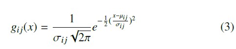
Considering a reference point P_i,  and  N  sensors S ₁, S ₂, …,  S _N , P_i’s Gaussian-based fingerprint can be expressed as a set of distributions FG = {g_i1(x), g_i2(x), …, g_iN (x)}. and the target, A is the RSSI measured at a reference distance from

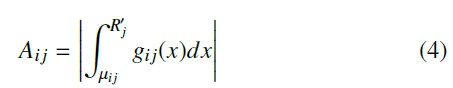
Given a set of RSSI measurements U = [R1, R2, …, RN ] from the target device, the penalty of matching U to FG can be estimated in two ways. The first is the area-under-the-curve (AUC) method, proposed by [7]. It computes the AUC (denoted as  A_{i j}) for each R′j under the Gaussian distribution g_{i j}(x), as shown in (4). The penalty of matching U to FG is approximated by the mean of all  A_{i j}. The smaller the mean over A_{i j}, the more likely the target device originates from reference point P_i.

After estimating device-to-sensor distances, we use least squares

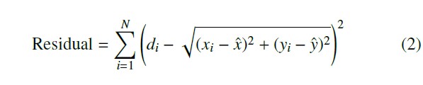
optimization to search for the coordinates (xˆ, yˆ) that minimize the residue in (2). In the equation, d_i is the estimated distance be- tween the target device and the i-th sensor; (x_i, y_i) represents the coordinates of the i-th sensor; and (xˆ, yˆ) represents the estimated coordinates of the target device.

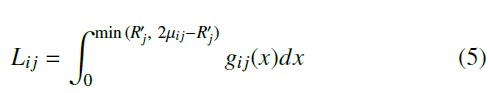
Our initial localization results show that Gaussian-based finger- printing with the AUC method does not perform well, especially when there is significant misalignment between some R′j and µ_{i j}. This is most likely due to the flaw of the penalty structure in the AUC  method (see Section 6.2 for details).  To  offer a better alternative, we propose the tail method, which uses tail probabilities to represent the likelihood that an individual R′j  originates from   g_{i j}(x). The product of all such individual likelihoods is the overall likelihood that U  matches FG .  Concretely, let L_{i j} be a likelihood

3.2 Fingerprinting

The concept of fingerprinting in active localization is described in Section 2.2. Similar to multilateration, the adaptation from active to passive localization only entails changing the manner in which RSSI is obtained, i.e., instead of measuring RSSI on the target device from signals sent by nearby APs, we measure RSSI on the nearby sensors from the signal sent by the target device.

We employ two methods to establish RSSI fingerprints. The first involves vector-based fingerprinting. We use RSSI vectors  as fingerprints, in which each value is the mean of all RSSI measurements obtained by a specific sensor at a given reference point [11]. For example, given N sensors S ₁, S ₂, …, S _N and M reference points P₁, P₂, …, P_M, we denote R_{i j1}, R_{i j2}, R_{i j3}, …, as the RSSI measurements emitted from reference point P_i (1 i M) and captured by sensor S _j  (1     j     N).  Let µ_{i j}  be the mean of R_{i j1}, R_{i j2}, R_{i j3}, …. The vector-based fingerprint of P_i can be written as FV = [µ_i1, µ_i2, …, µ_iN ].

When a target device generates a vector of RSSI measurements U = [R′1, R′2, …, R′N ] at an unknown location, the penalty of matching U to FV can be approximated by their Euclidean distance. The smaller the distance, the more likely the target device originates from reference point P_i.

The second method is Gaussian-based fingerprinting. It uses a set of Gaussian distributions as RSSI fingerprints, where each distri- bution corresponds to the RSSI measurements obtained by a specific sensor at a given reference point [7]. Extending the example above, Gaussian-based fingerprinting computes both the mean (µ_{i j}) and i estimator, which is the smaller of the two AUCs from the cumulative density functions extending from R′j to either tail of the distribution. Figure 1 illustrates the definition of L_{i j}. In the figure, R′j is placed in a Gaussian distribution g_{i j}(x), with mean µ_{i j} and standard deviation σ_{i j}. L_{i j} is the AUC from R′j  to the right tail.  The larger the value of L_{i j}, or the closer R′j is to µ_{i j}, the more likely R′j originates from g_{i j}(x).

RSSI

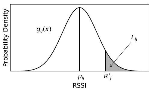
Figure 1: Tail Probability of R′j in a Gaussian Distribution g_{i j}(x)

L_{i j} can be written as (5). The penalty of matching U to  FG  can be approximated by the product over all L_{i j}, which is then con- verted to the sum of the negative logarithm of all L_{i j} to facilitate

computation. The smaller the sum, the more likely the target device originates from reference point P_i.

4        Data Collection

To evaluate the passive localization methods discussed in Section 3, RSSI measurements from mock probe requests, along with the

Once the penalty is obtained from the target device to all ref- erence points using either the vector- or Gaussian-based method, K-nearest neighbors is used to find the top k best-match reference points. The exact value of k is determined empirically via a valida- tion set. The average location of the top-k reference points is the predicted location of the target device.

3.3    Machine Learning-boosted Multilateration

We use the RSSI path-loss model in (1) to estimate distance based on RSSI measurement. However, (1) does not capture all the error terms [10]. While it is possible to create more complex path-loss models with add-on error terms, we can train a standard machine learning model to “learn” the relationship between RSSI measure- ments and distances, with error implicitly included. Machine learn- ing may capture relationships not explicitly described by a physical model. Thus, it is likely that a machine learning model will perform better than the idealized physical model in (1). We use three standard machine learning algorithms—multi-layer perceptron (MLP), sup- port vector machine (SVM), and k-nearest neighbors (K-NN)—to train regression models from RSSI measurements and distance at each sensor. Each model is then used to conduct multilateration, as described in Section 3.1.

environment. In the following sections, we present the experimental setup, experimental design, hardware details (sensor and emitter), field preparation, and data collection procedure.

4.1    Experimental Design

Figure 2(A) shows the layout of the testbed. Each cell is a 1 m by 1 m square, making the entire field 15 m by 15 m. Four sensors (red dots) s₁, s₂, s₃, and s₄ are placed at coordinates (0, 15), (15, 15), (0, 0), and (15, 0), respectively. During data collection, an emitter is placed on each data collection point (blue dots) and allowed to send approximately one-thousand mock probe requests. Each contains a Media Access Control (MAC) address that is traceable to a specific data collection point, distinguishable from a genuine probe request, and unique. After a mock probe request is captured by a sensor, the data is uploaded and stored in a database hosted on Amazon Web Services (AWS). Since four sensors are present in the testbed, at most four RSSI measurements are collected per probe request.

3.4          Machine Learning Classification of Reference Points

In fingerprinting, a set of RSSI measurements are passed to a fingerprinting algorithm as inputs, and the most likely reference point is returned as the localization output.  This process is similar to a machine learning classification model, where input features are RSSI measurements, and output labels are reference points. The difference between the two is that the former uses pre-specified rules to determine how RSSI measurements match reference points, whereas the matching is “learned” from training data in the latter. We apply the same machine learning algorithms (MLP, SVM, and K-NN) to train classifiers that map a set of RSSI measurements to the best-match reference point.

3.5          Machine Learning Regression of Coordinates

In [9], the authors offer a simple approach to performing active localization. They train a machine learning regressor that takes RSSI measurements and propagation delays of transmitted signals as input, and directly predicts the GPS coordinates of a target de- vice. Despite not having access to the propagation delay data, we can still adapt this approach to passive localization using the RSSI measurements alone. We follow the same setup as in Section 3.4, but instead of training a classifier, we train two regressors that take RSSI measurements as input and predict a reference point’s x- and y-coordinate, respectively. With the two regressors, we can directly estimate a target device’s location based on the RSSI measurements.

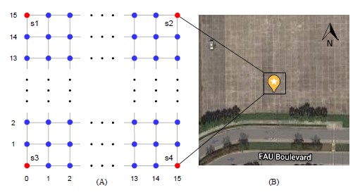
Figure 2: Experimental design and satellite view of the testbed

4.2          Hardware – Sensor

We used the same sensor described in [14]. It captures WiFi probe requests from the environment, removes duplicate MAC addresses at each 30-second window, and uploads aggregated data to AWS. In this paper, we added a new feature to differentiate mock probe requests from genuine probe requests, which allows the sensor to upload mock probe requests to a database dedicated to the exper- iment. The uploaded data include MAC address, time of capture, and RSSI measurement.

4.3          Hardware – Emitter

We used the same stress testing device described in [14] as the emitter of mock probe requests. It emits WiFi probe requests with a custom MAC address, on a specified channel, at a specified rate.

MAC address customization ensures traceability. The first four letters of the address are synced to the time of emission (timezone EST) in the format “HH:MM”. Since the timestamp at each data

collection point is recorded, a time-stamped MAC address encodes the location where the mock probe request was emitted. To ensure mock probe requests are distinguishable from genuine probe requests, the fifth and sixth positions of the address are fixed as “00”. A “HH:MM:00” prefix guarantees few, if any, collisions with genuine probe requests. Finally, to ensure that mock probe requests are unique among themselves, the remaining six positions are filled with random hexadecimals. As an example, a mock probe request emitted at 3:04 PM EST would have a MAC address similar to “15:04:00:1A:2B:3C”.

The MAC address customization is only traceable at the granularity of one minute. If two mock probe requests are emitted from different data collection points within the same minute of an hour, their locations cannot be distinguished (i.e. the first four letters of their MAC addresses would be identical). To avoid such complications, the emitter remains at each data collection point for at least a full minute before moving to the next. In the experiment, the emitter uses cronjobs to send approximately 1,000 mock probe requests in the first 50 seconds of each minute, and zero in the remaining 10.

4.4          Testbed Preparation

An empty outdoor area (GPS: 26.381488, -80.099640) with no nearby obstacles was used as the testbed to avoid complications in RSSI measurement. Figure 2(B) shows an overhead view of the field. Figure 3 provides a detailed view after the 15 m by 15 m grid has been prepared with spray chalk. The southwestern corner is chosen as the origin point of the field, with coordinates (0, 0).

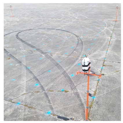
Figure 3: Mounted sensors on the testbed with grid drawn

The sensors were mounted on tripods, with an elevation of approximately 1.8 m above the ground. The four tripods were posi- tioned at s₁, s₂, s₃, and s₄, as illustrated in Figure 2. Three of the tripods are visible in Figure 3.

4.5          Data Collection Procedure

Data are collected by placing the emitter on each data collection point. The emitter is mounted on the same type of tripod as the sensor, but with an elevation of only 1 m. This mimics the height at which a WiFi-enabled device is likely to be carried by a pedes- trian. During the first 50 seconds of each minute, the emitter is left alone on the data collection point, without anyone present within the boundaries of the testbed. In the remaining 10 seconds, a researcher enters the field and moves the emitter to the next point. This setup ensures that signal transmissions are not affected by transient ob- structions. At each data collection point, the coordinates and the current timestamp are recorded. This procedure is repeated until all data collection points are visited.

Data collection for this manuscript was conducted from 15:00 to 20:00 on 2020-07-16.

5        Data Preparation

The raw probe request data contains 221,553 observations, one per mock probe request. Each observation contains five parameters, corresponding to the RSSI measurement (one per sensor) and timestamp. Observations with missing measurements are discarded. The resulting cleaned data set contains 171,537 observations. To further reduce the computation cost of model training, and to balance the number of observations across data collection points, 100 observations are randomly selected from each data collection point to form the sampled data set.

The sampled data set is one of the two data sets used in this paper. It contains 25,200 rows and 11 parameters. Each row corresponds to an individual mock probe request. The parameters correspond to four RSSI measurements (R₁ through R₄), coordinates of the data collection points (x and y), distances to each sensor (d₁ to d₄), and unique labels of the data collection points (label). Table 1 shows the structure of the sampled data set.

Table 1: Structure of the sampled data set

R₁…R₄              x        y              d₁…d₄     label

-44 … -41     0.0     1.0     14.0 … 15.0         16

-43 … -41     0.0     2.0     13.0 … 15.1         32

…                     …       …                      …          …

The other data set used in this paper is the mean data set, de- rived from the cleaned data set by taking the mean and standard deviation of RSSI measurements from each sensor at each data collection point. The mean data set contains 252 rows and 15 pa- rameters. Each row corresponds to a data collection point. The parameters correspond to four mean RSSI measurements (µ₁ to µ₄), coordinates of the data collection points (x and y), distances to each sensor (d₁ to d₄), four RSSI standard deviations (σ₁ to σ₄), and unique labels of the data collection points (label). Table 2 shows the structure of the mean data set.

Table 2: Structure of the mean data set

µ₁ … µ₄                    x        y            d₁ … d₄           σ₁ … σ₄      label

-44.3, …, -42.8    0.0     1.0     14.0 … 15.0     0.93 … 1.15        16

-44.1, …, -40.7    0.0     2.0     13.0 … 15.1     1.60 … 0.64        32

After random shuffling, the sampled data set is split into a sampled training set (80%, 20,160 observations) and a sampled testing set (20%, 5,040 observations) using scikit-learn [25]. The mean data set cannot undergo the same splitting procedure due to having only one observation per data collection point. Hence, the entire mean data set is treated as the mean training set (252 observations). Finally, the mean and standard deviation of RSSI measurements by each sensor at each data collection point from the sampled testing set form the mean testing set (252 observations).

The training sets are used exclusively for model training and validation. In particular, the sampled training set is used in all methods except fingerprinting; the models thus trained are called sampled models. The mean training set is used in all methods; the models thus trained are called mean models. The difference between sampled and mean models is that the former is tuned using the individual observations in a training set, whereas the latter is tuned by their mean values. It is worth noting that averaging RSSI measurements seems to have both positive and negative impacts on model performance, as it simultaneously reduces random error [2] and training size. It is thus interesting to study how the performance of the mean model compares to that of the sampled model.

All  data  preparation  procedures  were  conducted  using  the pandas Python library [26].  Figure 4 illustrates the relationships

6.1          Multilateration

Two RSSI path-loss models, one using the sampled training set and one using the mean training set, are created by linear regres- sion according to (1) for each sensor. The performance of the two models, evaluated on the sampled testing set, is shown in Table 3. The R2 score describes the amount of variance explainable by

the path-loss model, and the mean absolute error (MAE) describes the error between the estimated and actual distance. Within each sensor, the two models have almost identical performance. This means that averaging RSSI measurements does not alter model per- formance. Across the models of different sensors, s₄ has the best performance, whereas s₁  has the worst.  This may be explained  by a consistent source of interference from the northwest corner of the testbed. Since s₁ is closest to the northwest corner, it was affected the most. s₄  is furthest from the interference source,  so it was affected the least. However, the validity of this explanation cannot be verified until the same performance pattern repeats over time in future research.

Table 3: Metrics of the path-loss model

Sensor        Sampled              Mean

R2       MAE        R2       MAE

among the derived data sets, where their names, lineage, and shapes                                                                                                                                                             

(rows × columns) are shown.

s₁             0.61       4.62     0.61       4.63

s2	0.65	4.06            0.65	4.07
s3	0.61	4.03            0.61	4.03

100 random samples per reference point

Sampled Dataset 25,200

Raw Dataset 221,553

Exclude missing data

Take mean

Cleaned Dataset

171,537

Mean Training Set 252

1000 random samples

   s₄             0.71       3.44     0.71       3.46

Two multilateration models are generated, one based on the sam- pled RSSI path-loss model and the other based on the mean RSSI path-loss model. We first convert RSSI measurements to distances, and then pass the distance data to scipy’s least squares optimiza- tion API to estimate the target device’s coordinates [27]. Figure 5(A) demonstrates the localization performance of the traditional multilateration method. The x-axis denotes localization errors, and Sampled Training Set 20,160 Random split Mean Testing Set 252 Sampled Testing Set 5,040 Take mean Sampled Validation Set 1,000 the y-axis denotes the probability that a model’s localization error is smaller or equal to a selected x-axis value. The blue (sampled- sampled), orange (mean-sampled), and green (mean-mean) curves represent the localization performance under three scenarios: the sampled model tested on the sampled testing set, the mean model tested on the sampled testing set, and the mean model tested on the

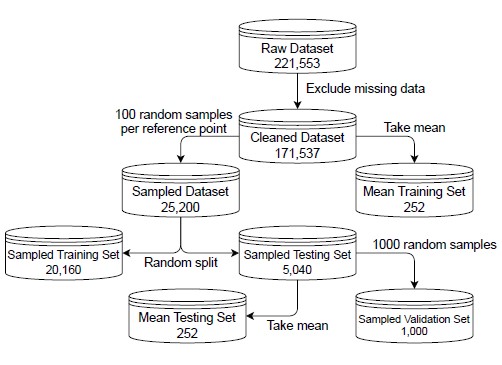
Figure 4: Relationship among all data sets

6 Traditional Methods

In this section, we present the adapted multilateration and finger- printing methods for passive localization and consider their per- formance. Here, localization performance is visualized by the cu-mean testing set, respectively.

The sampled-sampled curve does not show on the figure because it overlaps with the mean-sampled curve. This is expected because the sampled and the mean RSSI path-loss models have similar distance estimation performance. The mean-mean scenario performs slightly better than the other two. However, this is likely an artifact because the mean training and testing sets are very similar. Recall that the cleaned data set is the source of the mean training set, and the sampled testing set is the source of the mean testing set (Figure 4). Since the sampled testing set is a subset of the cleaned data set, the mean testing set shares information with the mean training set. The similarity between the mean testing and training sets inflates the measured performance of the mean-mean scenario.

6.2          Fingerprinting

The radio map for vector-based fingerprinting is a 252 4 matrix prepared from the mean training set, where each row represents a reference point, and each column represents the mean RSSI measure- ments from a sensor. As mentioned in Section 3.2, we empirically determine k, the number of top-match reference points that produces the best coordinate estimation. A series of fingerprinting models parameterized with different values of k are used to perform localiza- tion on a validation set. The k leading to the least validation error is selected. Usually, the validation set is withheld from the training set. However in fingerprinting, the mean training set, which is also the radio map, has no redundancy to supply a validation set. Therefore, we set aside 1,000 observations from the sampled testing set as the validation set (Figure 4). The observations in the validation set are not included in evaluating model performance. Validation error is defined as the root mean squared localization error, following [11].

Orange (v-mean-mean) curves represent localization performance when vector-based fingerprinting is tested on the sampled (excluding the validation set) and mean testing sets, respectively. Similar to traditional multilateration, the performance of v-mean-mean is better than that of v-mean-sampled. Again, this is most likely an artifact due to information overlap between the mean testing and training sets.

The radio map for Gaussian-based fingerprinting is a 252 4 matrix prepared from the mean training set, where each row repre- sents a reference point, and each column represents the Gaussian distribution, modeled from the mean and standard deviation of the RSSI measurements from the corresponding sensor. We follow the same procedure described above to find the best k, except that in the K-nearest neighbor API, (4) and the mean over A_{i j} are used for the AUC method, whereas (5) and the sum over negative loga- rithm of L_{i j} are used for the tail method. The result of the search shows that the minimum validation error is reached when k = 2 for both the AUC and the tail methods. Figure 5(B) shows the localization performance of Gaussian-based fingerprinting based on the optimal k value. The green (g-auc-mean-sampled) and red (g-auc-mean-mean) curves represent the performance under the AUC method, while the magenta (g-tail-mean-sampled) and brown (g-tail-mean-mean) curves represent the performance under the tail method. Both the g-auc-mean-sampled and g-tail-mean-sampled curves are based on the sampled (excluding the validation set) test- ing set, whereas both the g-auc-mean-mean and g-tail-mean-mean curves are based on the mean testing sets. The g-auc-mean-mean and g-tail-mean-mean curves again exhibit better performance than the g-auc-mean-sampled and g-tail-mean-sampled curves, respec- tively, which is likely an artifact.

Comparing performance across all curves (excluding the ones under mean-mean scenario), the vector-based fingerprinting (v- mean-sampled) performs the best. However, its lead over Gaussian- based fingerprinting under the tail method (g-tail-mean-sampled) is very modest.

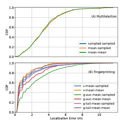
Figure 5: CDF curves of error in traditional methods

Comparing the two methods within Gaussian-based fingerprint- ing, the tail method consistently outperforms the AUC method. This is most likely due to the difference in penalty structure, where the AUC method, unlike the tail method, does not penalize misalign- ment proportionally to its severity. Figure 6(A) shows an example of how the penalty structure of the AUC method would fail to match a set of unknown RSSI measurements to the most probable finger- print. In the figure, a Gaussian-based fingerprinting radio map is visualized, which contains two reference points (P₁ and P₂), each fingerprinted by two sensors (S ₁ and S ₂). The two blue distribu-

We use scikit-learn’s K-nearest  neighbor  API  to  search for the optimal k. The API is called with default settings, except algorithm is set to brute, and n neighbors is set to k, which ranges from 1 to 20 for each validation run. For the data sets col- lected, we find that the validation error reaches its minimum when k = 2. Using this k, we evaluate the performance of vector-based fingerprinting; results are shown in Figure 5(B). The axis layout  is the same as described earlier. The blue (v-mean-sampled) and tions represent the RSSI fingerprint of P₁, denoted by the means [µ₁₁, µ₁₂]. Similarly, the two orange distributions represent the RSSI fingerprint of P₂, denoted by the means [µ₂₁, µ₂₂]. For simplicity, all distributions are assumed to have the same standard deviation. The set of unknown RSSI measurements, U = [R′1, R′2], are illustrated by two black dashed lines. Finally, the areas-under-the-curve used in the AUC method are labeled as A₁₁ and A₁₂ for P₁, and A₂₁ and A₂₂ for P₂. sum of their negative logarithms) further amplifies the misalignment penalty. In an extreme case, imagine that R′1 is perfectly aligned with µ₂₁ in Figure 6(B), and thus receiving the least amount of penalty. Yet, the severe misalignment between R′2 and µ₂₂ would still overwhelm the overall penalty for P₂ and readily make it a worse match than P₁. Therefore, the tail method is better-suited for Gaussian-based fingerprinting than the traditional AUC method; the difference in their localization performance is thus unsurprising.

7        Machine Learning Methods

Although it is clear that  P₁  is a better match for U  than  P₂,  it is not apparent in Figure 6(A). According to the AUC method described in Section 3.2, the match is selected as the smaller of A₁₁ + A₁₂ and A₂₁ + A₂₂. Due to the large misalignment between R′2 and both µ₁₂ and µ₂₂, we have A₁₂ A₂₂. Thus, the actual comparison is between A₁₁ and A₂₁, which does not yield a clear winner at first glance. However, the decision should not have been left to a comparison between A₁₁ and A₂₁ in the first place. The extreme misalignment between R′2   and µ₂₂ should have already disqualified P₂. The AUC method is unable to recognize this because its penalty structure is inversely proportional to the severity of RSSI misalignment (i.e., the amount of penalty per unit of misalignment decreases as misalignment becomes more severe). R′2 demonstrates how this penalty structure fails. While it is expected that a match between R′2 and µ₂₂ is penalized much more than a match between R′2 and µ₁₂, the actual penalty associated with the former (A₂₂) is almost the same as the penalty associated with the latter (A₁₂). Thus, the failure to proportionally penalize misalignment makes the AUC method ill-equipped for Gaussian-based fingerprinting.

On the contrary, Figure 6 (B) illustrates that the tail method can readily match U to P₁ as expected. The layout of Figure 6(B) is the same as Figure 6(A), except that the areas-under-the-curve are redefined and labeled as L₁₁ and L₁₂ for P₁, and L₂₁ and L₂₂ for P₂. According to the tail method described in Section 3.2, the match is selected as the smaller of lg(L₁₁) lg(L₁₂) and  lg(L₂₁)  lg(L₂₂). While L₁₁ and L₂₁ remain similar, the difference between L₁₂ and L₂₂ is large, with L₂₂ being virtually 0. As a result, lg(L₁₁)  lg(L₁₂) is easily smaller than  lg(L₂₁)  lg(L₂₂), which matches U  to  P₁. The reasons why the tail method works are two-fold. First, its penalty structure is proportional to the severity of RSSI misalign- ment, which ensures that larger misalignment receives exponentially more penalty. Second, multiplication of tail probabilities (or the

Three methods—machine learning-boosted multilateration, machine learning classification of reference points, and machine learning regression of coordinates—are evaluated for RSSI-based passive localization. Each method is approached using three standard ma- chine learning algorithms, MLP, SVM, and K-NN. Each model is trained on sampled and mean training sets to produce sampled and mean models, respectively.

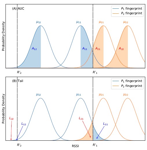
Figure 6: Example of matching under AUC or tail methods

During model training, we conduct two rounds of cross- validation to tune hyperparameters. For the sampled model, standard five-fold cross-validation is used. For the mean model, multi-fold cross-validation is not possible because the mean training set lacks sufficient redundancy. Thus, the same validation set discussed in Section 6.2 is used. In the first round of hyperparameter tuning, a wide range of values are provided, such that an optimal range can be identified for each hyperparameter. In the second round, values within each optimal range are used to find the exact hyperparameter values that minimize cross-validation error.

The finalized hyperparameter values are used to re-train the model, which is then subject to performance evaluation. The out-come of the evaluation is visualized as a CDF curve of the localization error in the same manner as described in Section 6. The sampled model is evaluated on the sampled testing set only, producing a sampled-sampled curve. The mean model is evaluated on both the sampled and mean testing sets, producing mean-sampled and mean-mean curves, respectively. As mentioned before, the validation set is excluded from evaluating the localization performance of the mean models.

All machine learning and hyperparameter tuning algorithms are executed using the corresponding APIs in scikit-learn.

7.1          Machine Learning-boosted Multilateration

 In machine learning-boosted multilateration, the RSSI path-loss model is replaced by a machine learning regressor to estimate dis- tance based on RSSI measurements. The advantage of this approach is that it assumes no prior knowledge of the complex RSSI-distance relationship and conducts regression without the constraints of a physical model.

Table 4: Metrics of machine learning RSSI-distance regressors

MLP                                            SVM                                                     K-NN

Sampled              Mean              Sampled              Mean              Sampled           Mean Sensor       R2       MAE        R2       MAE        R2       MAE                   R2       MAE        R2       MAE        R2       MAE

s1	0.53	2.48	0.52	2.50	0.53	2.45	0.53	2.47	0.52	2.48	0.53              2.48
s2	0.64	2.05	0.64	2.05	0.63	2.05	0.63	2.06	0.63	2.12	0.64              2.07
s3	0.57	2.39	0.56	2.40	0.56	2.35	0.55	2.36	0.57	2.39	0.56              2.44
s4	0.68	1.92	0.67	1.93	0.67	1.89	0.66	1.92	0.67	1.89	0.67              1.92

The hyperparameters tuned for the MLP regressor are hidden layer  sizes,  activation,  and  solver;  C,  kernel, and gamma for the SVM regressor; and n neighbors, weights, algorithm, and leaf size for the K-NN regressor. The maximum number of tuning iterations is 1,000 for the MLP, and 20,000 for the SVM and K-NN regressors.

Table 4 lists the R2 and MAE values for the machine learning RSSI-distance regressors after two rounds of hyperparameter tuning. Across machine learning algorithms, the sampled and mean models exhibit similar performance. Across sensors, s₄ exhibits the lowest error, whereas s₁ exhibits the highest error. This follows the results from the RSSI path-loss model. Comparing the performance between the machine learning and the RSSI path-loss models, we observe that the former consistently outperforms the latter in terms of MAE.

We use each machine learning RSSI-distance regressor to gener- ate its corresponding multilateration model as described in Section 6.1. Figures 7(A), (B), and (C) demonstrate their localization per- formance. Across all three machine learning algorithms, the models have similar performance, which is not surprising, given the similar performance in RSSI-distance regression mentioned above. The mean-mean curve performs slightly better, which, as described in Section 6, could be an artifact.

A comparison is also made among the best CDF curves across the three methods (mean-mean curve excluded), as shown in Figure 7(D). There is little difference in localization performance among them.

7.2          Machine Learning Classification of Reference Points

 

Machine learning classification is an alternative to the traditional fingerprinting method. A trained machine learning classifier takes four RSSI measurements from a target device as input and produces a predicted label as output. The label can be mapped to a refer- ence point, which is considered the estimated location of the target device.

The hyperparameters tuned for the MLP classifier are hidden layer sizes, activation, solver, and alpha;  C, kernel, gamma, and decision function shape for the SVM classifier;  and n neighbors,   weights,   algorithm,   and leaf size for the K-NN classifier. The maximum number of tuning iterations is 1,000 for all classifiers.

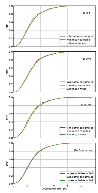
Figure 7: CDF curves of error in machine learning-boosted multilateration

Table 5: True and adjacent accuracy of machine learning classifiers

MLP                         SVM                        K-NN

Accuracy    Sampled                     Mean                     Sampled                     Mean                     Sampled                     Mean True                      0.63                                 0.55                                 0.70                                 0.68                                 0.69                                 0.68

Adjacent            0.81       0.78            0.84       0.83            0.84      0.80

1.0

0.8

0.6

0.4

0.2

0.0

1.0

0.8

0.6

0.4

0.2

0.0

1.0

0.8

0.6

0.4

0.2

sents the proportion of testing observations with correctly predicted labels. Adjacent accuracy denotes the proportion of testing observations with predicted labels that either match the true labels or one of the eight surrounding labels. The purpose of including adjacent accuracy is to reveal the degree of inaccuracy when a wrong prediction is made. Due to this intentional leniency, adjacent accuracy is always better than true accuracy. Across machine learning algorithms, the sampled model performs slightly better than the mean model. MLP performs the worst, whereas SVM and K-NN have similar performance.

Figures 8(A), (B), and (C) illustrate the localization performance of all three algorithms. Across machine learning algorithms, the sampled-sampled curve exhibits slightly better performance than the mean-sampled curve, but the mean-mean curve tops them both, with zero meter localization error more than 90% of the time. As discussed earlier, the exceptional performance exhibited by the mean-mean curve is most likely an artifact. However, the exaggeration in classification is much more pronounced than in multilateration. This is due to the way we compute localization errors for classifiers. Since we consider a correct match to a reference point as being equivalent to zero meter localization error, we accumulate many zero-error instances when evaluating the localization performance of classifiers. These zero-error instances inflate the CDF curves. In contrast, multilateration methods never exhibit zero meter localization errors.

We also compare the best CDF curves across the three machine learning algorithms, with the mean-mean curves excluded. Figure 8(D) shows the results, where SVM performs slightly better than the others.

7.3          Machine Learning Regression of Coordinates

Machine learning regression of coordinates trains two RSSI- coordinate regressors based on the x- and y-coordinates, respec- tively. It allows direct quantitative estimation of a target device’s position. Each regressor takes four RSSI measurements from an observation as input and produces a pair of estimated coordinates as output.

The hyperparameters tuned for the MLP regressor are hidden layer sizes, activation, solver, and alpha;  C, kernel, and gamma for the SVM regressor; and n neighbors, weights, algorithm, and leaf size for the K-NN regressor. The Table 5 lists the true and “adjacent” accuracy of each classifier after two rounds of hyperparameter tuning. True accuracy repre- maximum number of iterations is 1,000 for the MLP regressor, and 20,000 for the SVM and KNN regressors.

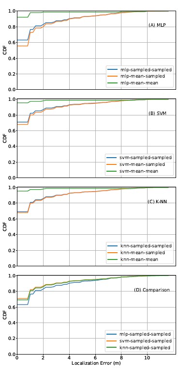
Figure 8: CDF curves of error in machine learning classification

Table 6: Metrics of machine learning RSSI-coordinate regressors

MLP                                            SVM                                                     K-NN

Sampled              Mean              Sampled              Mean              Sampled           Mean Coordinate       R2       MAE        R2       MAE        R2       MAE                           R2       MAE        R2       MAE        R2       MAE

x	0.84	1.24	0.83	1.30	0.91	0.71	0.82	1.29	0.91	0.71	0.88	0.97
y	0.86	1.16	0.85	1.24	0.90	0.74	0.85	1.21	0.91	0.71	0.90	0.80

RSSI-coordinate regressors after two rounds of hyperparameter tun- ing. Across all regressors, the sampled model has better regression performance than the mean model, which is likely due to the differ- ence in training size. However, it is worth noting that the difference in training set size does not affect the performance of the RSSI- distance regressors (Section 7.1). A possible explanation of why the RSSI-coordinate regressor is more sensitive to training set size is that it is a more complex model (four features as input) than the RSSI-distance regressor (one feature as input). Across algorithms, the sampled models of SVM and K-NN perform slightly better than that of MLP, while the mean model of K-NN outperforms that of MLP and SVM. Between the two coordinates, y-coordinates gener- ally have lower estimation error than x-coordinates. We speculate that this is the result of how our testbed is prepared, where there is more measuring variability in the x- versus y-axis.

Figures 9(A), (B), and (C) summarize the localization perfor- mance of all three algorithms. Within MLP and K-NN, the sampled- sampled curve performs slightly better than the mean-sampled curve, but the mean-mean curve outperforms both. This aligns with our earlier hypothesis that indicates performance exaggeration in the mean-mean curve. However, in the SVM models, the situation is surprisingly reversed. The sampled-sampled curve shows better performance than the exaggerated mean-mean curve. This is most likely due to the superior RSSI-coordinate regression performance of the SVM sampled model compared to the SVM mean model.

We then compare the performance of the best CDF curves across the three machine learning algorithms (excluding the mean-mean curves), as shown in Figure 9(D). The results show that the sampled- sampled SVM model performs the best.

8        Royal Rumble

To find the best-performing model overall, we juxtapose the best model within each method (excluding the mean-mean curves) in the same plot. If multiple models show equally good performance within a particular method, a model is arbitrarily selected. The result is shown in Figure 10. The axes are the same as before. The blue curve corresponds to the best performant model in traditional multi- lateration (sampled-sampled); the orange curve corresponds to the best in traditional fingerprinting (v-mean-sampled); the green curve corresponds to the best in machine learning-boosted multilateration (mlp-sampled-sampled); the red curve corresponds to the best in machine learning classification of reference points (svm-sampled- smapled); and the purple curve corresponds to the best in machine learning regression of coordinates (svm-sampled-sampled). Several observations can be made.

First, the best machine learning models outperform the best traditional models. Specifically, machine learning-boosted multilat- eration performs better than its traditional counterpart. Similarly, machine learning classification performs better than traditional fin- gerprinting. This is not surprising because machine learning meth- ods can train regressors and classifiers based on RSSI measurements without the constraints imposed by an underlying physical model. It allows them to capture patterns that might be ignored in the traditional methods.

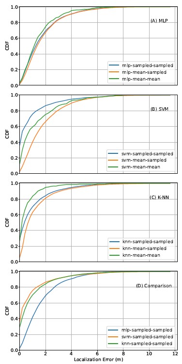
Figure 9: CDF of error with machine learning RSSI-coordinate regression

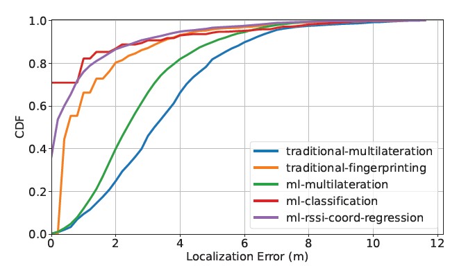
Figure 10: The best CDF curves of error among all methods

Table 6 lists the R2 and MAE values for the machine learning Second, the best non-multilateration models outperform the best multilateration models by a wide margin. This is most likely due to the nature of the multilateration methods, where two rounds of esti- mation are involved: RSSI to distance and distance to coordinates. Since each round of estimation incurs error, the multilateration methods accumulate more error than the other methods, where only one round of estimation is involved.

Third, except for fingerprinting, where there is no sampled- sampled option, all of the CDF curves used for comparison in Figure 10 are sampled-sampled curves. In other words, given the same sampled testing set, the sampled models either outperform or perform as well as the mean models for all methods. This result answers the question raised at the close of Section 5: The benefit of reduced random error in the mean training set does not outweigh the costs of reducing the size of the training set.

Finally, for a localization model to function at the scale of a city street, its error must be below a certain threshold. Ideally, the error should be small enough to tell whether a target device has moved from one business to another. Based on this reasoning, the best ma- chine learning classifier (svm-sampled-sampled), the best machine learning RSSI-coordinate regressor (svm-sampled-sampled), and the best traditional fingerprinting (v-sampled-sampled) are the best candidates, as they all exhibit above 90% probability of having four meters or less localization error. However, future research must examine their spatial robustness (e.g., does the model work outside the testbed?) and temporal robustness (e.g., does the model work on data collected a week or a month later?).

9    Conclusion

In this paper, we have systematically evaluated the localization performance of several RSSI-based passive localization methods using data collected in a semi-controlled, obstruction-free outdoor environment. The methods include two adaptations of traditional active localization methods (multilateration and fingerprinting) and three machine learning methods (machine learning-boosted multi- lateration, machine learning classification of reference points, and machine learning regression of coordinates). The results show that the machine learning methods perform better than the traditional methods. Further, the SVM sampled model in the classification- based approach, the SVM sampled model in the RSSI-coordinate regression-based approach, and the traditional fingerprinting ap- proach seem to have sufficiently good performance to be considered for use in real-world mobility monitoring. However, several limita- tions in formulating and evaluating these methods must be addressed and improved upon in future research.

First, all the models in this paper are trained and tested on data collected in a five-hour window on the same day. In practice, we have documented and verified that RSSI measured under identi- cal emitter, sensor, and visible environmental conditions exhibits temporal variability [28]. Thus, a localization model must possess temporal robustness such that the time of data collection is irrele- vant to its performance. Further, the exceptional performance of the mean-mean curves in almost all models appears to be an artifact due to the information overlap between the mean testing and training sets. It will be interesting to see whether the mean-mean curves remain exceptional when the mean testing set comes from data col- lected during a different session. Future research will pursue this evaluation.

In addition, the data used in this paper were collected in a near- ideal environment, free of obstructions and adverse weather events. We have yet to include samples with missing data in the analysis (e.g., three instead of four RSSI measurements in a sample). How- ever, signal noise and incomplete data are inevitable in practice. Thus, future research will investigate how model performance de- teriorates when data are collected with missing features (e.g., not all sensors capture a probe request), under unfavorable weather conditions (e.g., rain), in the presence of obstructions (e.g., walls, people), or with interference from other devices.

Relatedly, all the models trained in this paper are based on data collected by exactly four sensors. This presents a scalability issue, in which the addition or removal of a few sensors could require model re-training. Since scaling sensor deployments up and down is not uncommon, future research will focus on generating models resistant or adaptable to small changes in sensor availability.

Conflict of Interest

The authors declare no conflict of interest.

Acknowledgment

This research is supported by the City of West Palm Beach, the Knight Foundation, and the Community Founda- tions of Palm Beach and Martin Counties. The authors would like to thank Chris Roog, Executive Director of the Community Redevel- opment Agency in the City of West Palm Beach, for his continued assistance and support in realizing MobIntel; and thank the Florida Atlantic University I-SENSE team for providing hardware, software, and logistics support. This work was partially supported through the NSF ERC for Smart StreetScapes (CS3) (EEC-2133516).

1. L. Sun, S. Chen, Z. Zheng, L. Xu, “Mobile Device Passive Localization Based on IEEE 802.11 Probe Request Frames,” Mobile Information Systems, 2017, 1–10, 2017, doi:10.1155/2017/7821585.
2. W. Xue, W. Qiu, X. Hua, K. Yu, “Improved Wi-Fi RSSI Measurement for Indoor Localization,” IEEE Sensors Journal, 17(7), 2224–2230, 2017, doi: 10.1109/JSEN.2017.2660522, conference Name: IEEE Sensors Journal.
3. K. K. Mamidi, K. P. V., “ALTAR: Area-based Localization Techniques using AoA and RSS measures for Wireless Sensor Networks,” in 2019 International Conference on contemporary Computing and Informatics (IC3I), 160–168, 2019, doi:10.1109/IC3I46837.2019.9055582.
4. X. Li, Z. D. Deng, L. T. Rauchenstein, T. J. Carlson, “Contributed Review: Source-localization algorithms and applications using time of arrival and time difference of arrival measurements,” Review of Scientific Instruments, 87(4), 041502, 2016, doi:10.1063/1.4947001, publisher: American Institute of Physics.
5. G. Guo, R. Chen, F. Ye, X. Peng, Z. Liu, Y. Pan, “Indoor Smartphone Localiza- tion: A Hybrid WiFi RTT-RSS Ranging Approach,” IEEE Access, 7, 176767– 176781, 2019, doi:10.1109/ACCESS.2019.2957753, conference Name: IEEE Access.
6. N.-S. Duong, T.-M. Dinh, “Indoor Localization with lightweight RSS Fin- gerprint using BLE iBeacon on iOS platform,” in 2019 19th International Symposium on Communications and Information Technologies (ISCIT), 91– 95, 2019, doi:10.1109/ISCIT.2019.8905160, iSSN: 2643-6175.
7. C.-H. Lin, L.-H. Chen, H.-K. Wu, M.-H. Jin, G.-H. Chen, J. L. Gar- cia Gomez, C.-F. Chou, “An Indoor Positioning Algorithm Based on Fin- gerprint and Mobility Prediction in RSS Fluctuation-Prone WLANs,” IEEE Transactions on Systems, Man, and Cybernetics: Systems, 1–11, 2019, doi: 10.1109/TSMC.2019.2917955, conference Name: IEEE Transactions on Sys- tems, Man, and Cybernetics: Systems.
8. J. Wang, J. Luo, S. J. Pan, A. Sun, “Learning-Based Outdoor Localization Exploiting Crowd-Labeled WiFi Hotspots,” IEEE Transactions on Mobile Com- puting, 18(4), 896–909, 2019, doi:10.1109/TMC.2018.2849416, conference Name: IEEE Transactions on Mobile Computing.
9. L. L. Oliveira, L. A. Oliveira, G. W. A. Silva, R. D. A. Timoteo, D. C. Cunha, “An RSS-based regression model for user equipment location in cellular net- works using machine learning,” Wireless Networks, 25(8), 4839–4848, 2019, doi:10.1007/s11276-018-1774-4.
10. Z. He, Y. Li, L. Pei, R. Chen, N. El-Sheimy, “Calibrating Multi-Channel RSS Observations for Localization Using Gaussian Process,” IEEE Wireless Com- munications Letters, 8(4), 1116–1119, 2019, doi:10.1109/LWC.2019.2908397, conference Name: IEEE Wireless Communications Letters.
11. S. Yiu, M. Dashti, H. Claussen, F. Perez-Cruz, “Wireless RSSI fingerprinting localization,” Signal Processing, 131, 235–244, 2017, doi:10.1016/j.sigpro. 2016.07.005.
12. R. Sari, H. Zayyani, “RSS Localization Using Unknown Statistical Path Loss Exponent Model,” IEEE Communications Letters, 22(9), 1830–1833, 2018, doi:10.1109/LCOMM.2018.2849963, conference Name: IEEE Communica- tions Letters.
13. S. Sadowski, P. Spachos, “RSSI-Based Indoor Localization With the Internet of Things,” IEEE Access, 6, 30149–30161, 2018, doi:10.1109/ACCESS.2018. 2843325, conference Name: IEEE Access.
14. S. Mazokha, F. Bao, J. Zhai, J. Hallstrom, “MobIntel: Sensing and Analytics Infrastructure for Urban Mobility Intelligence,” in 2020 IEEE International Conference on Smart Computing (SMARTCOMP) (SMARTCOMP 2020), Bologna, Italy, Italy, 2020.
15. F. Bao, S. Mazokha, J. O. Hallstrom, “MobIntel: Passive Outdoor Localization via RSSI and Machine Learning,” in 2021 17th International Conference on Wireless and Mobile Computing, Networking and Communications (WiMob),
    247–252, 2021, doi:10.1109/WiMob52687.2021.9606338.
16. D. Alshamaa, F. Mourad-Chehade, P. Honeine, “Mobility-based Tracking Using WiFi RSS in Indoor Wireless Sensor Networks,” in 2018 9th IFIP In- ternational Conference on New Technologies, Mobility and Security (NTMS), 1–5, 2018, doi:10.1109/NTMS.2018.8328704, iSSN: 2157-4960.
17. H. Du, C. Zhang, Q. Ye, W. Xu, P. L. Kibenge, K. Yao, “A hybrid outdoor localization scheme with high-position accuracy and low-power consumption,” EURASIP Journal on Wireless Communications and Networking, 2018(1), 4, 2018, doi:10.1186/s13638-017-1010-4.
18. M. Youssef, M. Mah, A. Agrawala, “Challenges: device-free passive local- ization for wireless environments,” in Proceedings of the 13th annual ACM international conference on Mobile computing and networking, MobiCom ’07, 222–229, Association for Computing Machinery, New York, NY, USA, 2007, doi:10.1145/1287853.1287880.
19. J. Wilson, N. Patwari, “Radio Tomographic Imaging with Wireless Net- works,” IEEE Transactions on Mobile Computing, 9(5), 621–632, 2010, doi: 10.1109/TMC.2009.174, conference Name: IEEE Transactions on Mobile Computing.
20. G.-l. Wang, X.-b. Hong, X.-m. Guo, Y. Fang, “A Data-Driven Three- Dimensional RSS Model for Device-Free Localization and Tracking,” in 2019 IEEE 21st International Conference on High Performance Computing and Com- munications; IEEE 17th International Conference on Smart City; IEEE 5th In- ternational Conference on Data Science and Systems (HPCC/SmartCity/DSS), 1705–1713, 2019, doi:10.1109/HPCC/SmartCity/DSS.2019.00233.
21. A. Guillen-Perez, M.-D. Cano, “Counting and locating people in outdoor environments: a comparative experimental study using WiFi-based passive methods,” ITM Web of Conferences, 24, 01010, 2019, doi:10.1051/itmconf/ 20192401010, publisher: EDP Sciences.
22. T. Kulshrestha, D. Saxena, R. Niyogi, J. Cao, “Real-Time Crowd Monitoring Using Seamless Indoor-Outdoor Localization,” IEEE Transactions on Mobile Computing, 19(3), 664–679, 2020, doi:10.1109/TMC.2019.2897561, confer- ence Name: IEEE Transactions on Mobile Computing.
23. J. Du, C. Yuan, M. Yue, T. Ma, “A Novel Localization Algorithm Based on RSSI and Multilateration for Indoor Environments,” Electronics, 11(2), 2022, doi:10.3390/electronics11020289.
24. F. Shang, W. Su, Q. Wang, H. Gao, Q. Fu, “A Location Estimation Algorithm Based on RSSI Vector Similarity Degree,” International Journal of Distributed Sensor Networks, 10(8), 371350, 2014, doi:10.1155/2014/371350, publisher: SAGE Publications.
25. F. Pedregosa, G. Varoquaux, A. Gramfort, V. Michel, B. Thirion, O. Grisel, M. Blondel, P. Prettenhofer, R. Weiss, V. Dubourg, J. Vanderplas, A. Passos,
    D. Cournapeau, M. Brucher, M. Perrot, E. Duchesnay, “Scikit-learn: Machine Learning in Python,” Journal of Machine Learning Research, 12, 2825–2830, 2011.
26. Wes McKinney, “Data Structures for Statistical Computing in Python,” in Ste´fan van der Walt, Jarrod Millman, editors, Proceedings of the 9th Python in Science Conference, 56 – 61, 2010, doi:10.25080/Majora-92bf1922-00a.
27. P. Virtanen, R. Gommers, T. E. Oliphant, M. Haberland, T. Reddy, D. Cour- napeau, E. Burovski, P. Peterson, W. Weckesser, J. Bright, S. J. van der Walt, M. Brett, J. Wilson, K. Jarrod Millman, N. Mayorov, A. R. J. Nel- son, E. Jones, R. Kern, E. Larson, C. Carey, ˙I. Polat, Y. Feng, E. W. Moore, J. Vand erPlas, D. Laxalde, J. Perktold, R. Cimrman, I. Henriksen, E. A. Quintero, C. R. Harris, A. M. Archibald, A. H. Ribeiro, F. Pedregosa, P. van Mulbregt, S. . . Contributors, “SciPy 1.0: Fundamental Algorithms for Sci- entific Computing in Python,” Nature Methods, 17, 261–272, 2020, doi: https://doi.org/10.1038/s41592-019-0686-2.
28. S. J. Pan, V. W. Zheng, Q. Yang, D. H. Hu, “Transfer Learning for WiFi-based Indoor Localization,” AAAI Conference on Artificial Intelligence, 6, 2008.

(Click Here)