1. Introduction

This paper is an extension of work originally presented in the Fifth Conference on Cloud and Internet of Things (CIoT) [1]. By adding other methods such as the Genetic Algorithm, First-Fit, Random-Fit, and Simulated Annealing, our approach will predict the energy consumed by the data centers and the workload placement (containers) in the servers, offering best and optimal solutions to reduce energy consumption, waste of cloud resources, and have an energy-efficient container placement policy.

Generally, Cloud Computing is based on a large data center (server farm), in which many servers are connected to achieve high performance. The data centers represent an infrastructure of several instances (hosts, virtual machines…) [2]–[4]. Each of these instances requires an allocation at the data center because of the growing demand for hosting services. For these reasons, they are considered to be heavy consumers of resources and energy [3]. In data center, the energy consumed by active servers represents a large proportion of the total energy [4], [5]. More clearly, the energy consumed by the hosts or hosting servers plus network and storage equipment represents about 40% of the total energy [6]–[8]. Cooling equipment uses between 45% and 50% of the total energy, and the rest is shared among other systems such as lighting [6]–[11].

With the energy of the cooling systems, the costs in the data centers are experiencing a big explosion, which require a reduction in their expenses [12]. According to [5][9][13], the main challenges in data centers are to minimize the heat and energy consumed by cloud infrastructures and to secure them against threats.

So, to optimize the use of energy in data centers, it is necessary to define the servers that must be active according to the current workload and to avoid traditional techniques that negatively influence the quality of services (QoS) such as stopping components or reducing their performance [6], [9], [10]. In most data centers, the consumption of hardware and software resources of each active physical machine is between 11% and 50% with power consumption between 50% and 70% compared to a server whose resources are used entirely by the hosting of the instances and applications executed on these instances [2], [9], [14]. For this, the efficient placement of virtual instances is very important to control the use of material resources and prohibit any kind of their waste that can lead to an increase in energy consumption.

Our approach will have two objectives. The first will be the prediction of workload placement using the Genetic Algorithm and the First Fit Decreasing to define a better placement of a new type of virtual instance called containers. This placement will be constrained to define the best lower number of servers to host container instances. The second objective is the main one, which will be the prediction of energy consumed by a data center, by applying our container placement algorithms to have the best solutions in terms of reducing the energy consumed by a data center and optimizing the use of hardware resources such as RAM, Storage, Bandwidth, etc.

The remainder of this paper is coordinated as follows. We present the related works in the second section. In the third section, we propose our methodology. We perform our algorithms in the fourth section, and the paper is concluded in section five.

2. Related Work

The estimation or prediction of energy consumption in data centers has become a necessary operation in recent years. Due to the huge growth in user demands for cloud services, the number of servers has started to increase to provide the necessary hardware resources. This implied an increase in energy consumption, which forced large cloud companies to do studies on the energy consumed by their data centers, to optimize it in the future, or replace their power source with a cheaper and guaranteed one.

In this context, several approaches estimate energy consumption in data centers. Most of these methods focus on servers to estimate energy. Each server or host is a set of resources such as RAM, HDD, and CPU. In this case, the energy of the host is relative to the sum of the power of all its resources, or according to some [15][16]. Mathematically, the energy consumed by a host is represented in the literature by linear functions that depend on a resource like CPU [15][17], or non-linear, whose functions are quadratic of the CPU resource use [17][18]. Heuristics and metaheuristics are methods that are widely used to estimate the energy in data centers based on the placement of virtual instances in servers especially metaheuristics as they are adaptive for complex problems that require considerable calculation.

In [19], they proposed the placement of virtual machines based on energy consumption by the resources of the data center. One of the objectives of this approach was to reduce energy consumption using a simulated annealing algorithm. This technique generates an initial solution called initial configuration which contains the placement of the VMs in servers, on which they applied at each iteration one of the three simulated annealing techniques: inversion, translation, and switching, to get the next configuration. To define which solution is better, they calculate the energy consumed by the data center in both cases and choose the one that gives the small energy value that will be the best solution. The disadvantages of this approach are the execution time which is very long for large instances, and its process ends if it finds that a new configuration is better than the previous one even if they remain several iterations. This decision does not necessarily indicate that the new configuration is the best among all other solutions.

The same thing in [20], they used the simulated annealing algorithm to propose an economic placement in terms of energy for virtual machines. The proposed algorithm goes through the four stages of the simulated annealing (generation of the initial configuration, obtaining the next generation, definition of the objective function, and timing of temperatures and evolution time). The simulated annealing proposed was compared by the First Fit Decreasing multi-start random searching approach. The results obtained show the effectiveness of the proposed method, but in the case of large instances, it takes a lot of time to find the best solution. For this, they used a time limiter to stop the calculation process in a solution very close to the best.

Other researchers have proposed multi-objective metaheuristics for the placement of workloads in servers by calculating the energy consumed by data centers, to select the best placement in terms of energy minimization. In [21], the authors used the multi-objective genetic algorithm to provide virtual machine placement by minimizing energy consumption and improving the quality of services and the use of resources. The contradictory nature of the objectives defined in this approach has necessarily influenced the distribution of the load between the resources in a data center.

The same thing in [22] and [23], which proposed an approach based on the ant colony algorithm to calculate and minimize the energy consumed by a cloud system based on the placement of virtual machines. In [23], they built a mechanism for measuring indirect energy consumption for virtual machines based on a model for calculating the energy consumed by these machines deployed in [24], because it is difficult to deduce the energy consumption directly from the material because of the existence of the virtualization technology.

Our approach will be different from the old works because we will use cloud containers instead of virtual machines. More of this, we will propose a genetic algorithm and a First-Fit-Decreasing algorithm to provide best container placement without wasting the resources of active servers, with the prediction of energy consumed by any data center to define which algorithm offers best and optimal solutions for the minimization of energy consumed and the optimization of material resources.

3. Methodology

Our main objective is to predict the energy consumed in a data center for a given workload using the genetic algorithm and FirstFit-Decreasing to predict the best or optimal placement of this load (cloud containers). The best algorithm will be one that offers optimal solutions in terms of minimizing energy consumption and optimizing the use of the hardware resources of a data center operating in a specific context.

3.1. Workload Placement

The placement of workloads is an operation that has a great impact on several problems in cloud computing such as minimizing energy consumption. The concept of this placement is to define the servers that will be active to host several virtual instances. To have an optimal placement, it is necessary to choose an optimal number of servers without wasting the material resources of the data center.

The workloads in our approach will be the containers. Containers are small virtual instances in terms of hardware and software resources [25]–[27]. They provide a virtual platform such as Docker, with which multiple users can drive and run their applications or images of operating systems directly on the physical machine [27], [26].

The containers are efficient compared to the virtual machines because they are lightweight and their installation takes a few seconds and they run directly on the operating system and the hardware of the physical machine. On the other hand, virtual machines take a long time to install and require hypervisors to run [26][25]. In [26], the author represents a containerization technology for creating container instances. It allows users to deploy and run their applications in process containers.

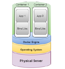
Figure 1: Operation of a container

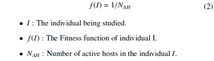
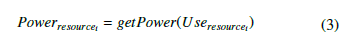
Our approach will propose two algorithms to predict the best and optimal placement for containers. The main objective will be the choice of an optimal number of servers sufficient to host the containers according to their material resources. This objective is defined by the following equation:

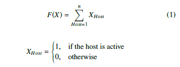
To achieve this goal, we have identified three necessary constraints. First, each container must have a placement at the end. The second constraint insists that each container must be placed in a single host. The latter checks that all containers must not exceed the host regarding material resources. For example, for RAM, we have decided to reserve 80% of each active host for container placement and keep the rest for user processing, ensuring proper load balancing between servers.

3.1.1     Genetic Algorithm

The genetic algorithm [28] is an optimization method (metaheuristic) [29] first presented by John Holland in the 1970s. It is based on techniques derived from genetics and the evolutionary mechanisms of nature: crossover, mutation, and selection.

It represents a method for solving complex optimization problems, with or without constraints, based on a natural selection process (a process similar to that of biological evolution). More precisely, it provides solutions to problems that don’t have calculable solutions in a reasonable time analytically[30][28].

The process of the genetic algorithm begins with the random creation of thousands of more or less good solutions, then they will be subjected to an evaluation to select the most suitable ones according to constraints. The population continues to evolve through the creation of other generations, by crossing the best solutions between them and having them mutate, then they are brought together with the best already chosen in the selection. This process will be restarted in a certain number of iterations to arrive at the best solutions.

Generation of the initial population: The genetic algorithm in its nature is a population-based method, i.e., it begins with a set of initial solutions named the initial population, and in each iteration, it produces a new generation of solutions of the same size as the initial one. To have an initial population, it must be generated from a set of solutions, which are called individuals (chromosomes). The total number of individuals generated represents the size of the population.

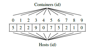
Figure 2: Representation of a chromosome (individual)

So to generate the initial population, you have to create a set of chromosomes as in the figure 3. This generation will be random within the constraints of the approach to ensure that each respects all the constraints of the problem to have a correct initial population.

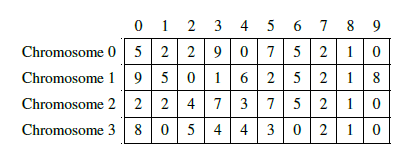
Figure 3: Representation of the structure of an initial population

Selection: For our approach, we decided to set the number of chromosomes in four for the initial population and the one to be built in each iteration and select the two best individuals (parents) among each created population, on which the crossing operator will apply to have two new individuals (sons) to build a new generation with new features. The selection of the best individuals is based on a criterion called the Fitness function. It is an equation defined according to the problem studied, to determine the best solutions that satisfy this function.

To determine the best individuals, we have based on the principle of our objective which serves to minimize the number of active hosts. More clearly, if a chromosome of a population respects all the constraints of the problem and contains the minimum possible hosts, then it represents a good solution among those in the studied population. This choice makes it possible to calculate the number of active hosts in an individual and choose two individuals which contain the minimum number of hosts, or the reciprocal of the number of active hosts, and then choose the two large values obtained. We represent below the equation of the Fitness function to select the best individuals.

The Fitness function will be applied at the beginning of the initial population to determine the individual parents, who will be the inputs of the next phase (the crossover). This function will be applied to each new generation created until the last iteration. These kinds of individuals, who represent the parents are feasible (workable) solutions for the problem studied. Workable individuals are solutions that met the needs of a problem.

So, the individual (parents) selected according to the Fitness function in each iteration are feasible solutions among others to discover probably in the following iterations. But instead of choosing both parents, we decided to compare them by choosing the best among them (the one that has the greatest value of Fitness, if they have equal values, then both will be chosen as feasible solutions). And each feasible solution represents one of the best-suggested ways to place containers in a minimum number of hotels without any waste of resources or energy consumed.

Crossover: The choice of the best individuals in the selection phase is the starting point of the crossover. These selected individuals are genetically better according to the function of Fitness, and they contain characteristics that will improve each population by producing new individuals called sons. The creation of new individuals is done by a crossover applied to the parents explained by the following two points:

• Divide each parent individual into two parts (from the middle), if the size of the individual is even, then both parts will have the same length, otherwise, the first part will exceed the size of the second with an element.
• Concatenate the first part of the first parent with the second of the other to have the first son, then the second part of the first parent with the first of the other parent to have the second son.

After creating the new individuals (sons), the parent individuals are kept to build a new generation of four chromosomes as the initial population after the application of the mutation operation on the sons. Keeping parents is not optional, but it has two very important roles in the algorithm process.

First, it avoids the case of having a bad generation, because parents are already good solutions according to the Fitness function applied in the selection, on the other hand, there is no information about the nature of new individuals created, whether they are good solutions to the problem or not, until the application of the mutation phase and build a new population and apply the selection operator to it to indicate the individuals who will be the new parents who may be one of the created sons of the previous iteration or both or none.

Secondly, the conservation of parents and combining them with the new individuals makes it possible to respect the rule of construction of a population in the genetic algorithm which indicates that all generations must be of the same size as the one at the beginning, as well as this combination guarantees diversity in the best solutions and increase the proportion of having several that are feasible.

Mutation: Generally, the mutation principle is used to apply more change to the sons created in the crossover phase to obtain a rich and different population from the previous one. These changes will apply to some genes of one or more chromosomes. In our case, the genes on each chromosome are the identifiers of the hosts chosen to host the containers, as shown in the figure 4.

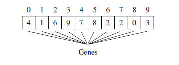
Figure 4: Individual-level active hosts represent their genes

So the change in the hosts of an individual involves a modification in the location of the containers. For this reason, the mutation phase for our approach will be slightly different compared to those of other problems that use the genetic algorithm. More precisely, The main role of the mutation will be corrective, that is to correct the faults produced by the crossing at the level of the son individuals. This crossing can cause false locations for containers at these individuals. For this reason, we must first check the location of the containers in each child’s individual if one or more exceed the host that hosts them in terms of RAM. In this way, the two sons will be corrected by ensuring that they respect the constraints of the approach before combining them with the parents to build a new generation.

This ”corrective” mutation has another impact because the correction made at the level of the sons will have a great chance of bringing back new characteristics. After all, the containers in those chromosomes have probably different locations to those in the individual parents, and therefore the possibility of having other better solutions. With all these characteristics, the mutation phase will have a great impact on the realization of a good dynamic container placement which is one of the big goals of this optimization problem, meaning the appearance of the migration notion of virtual instances between active hosts, which is absent in the static placement which prevents the migration of a container from one host to another after having placed it.

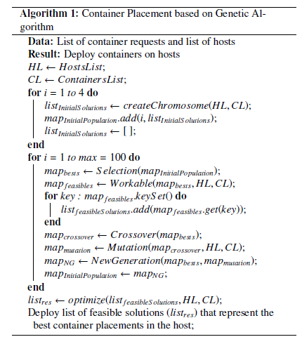
Deploy list of feasible solutions (list_res) that represent the best container placements in the host; Algorithm 1 shows the principle of the genetic algorithm and the main methods used to achieve the objective of the problem. Input data is set before starting initialization. This entry will help the different operations related to the algorithm to determine the possible feasible solutions that will be the result, which represent several best container placements.

The algorithm starts by checking the selected input data, which are the hosts and the containers to be placed. This operation checks whether the total sum of Rams of all outbound hosts is greater than that of containers, to ensure that there is sufficient space for the placement of the container request. Then, if the verification is done and the input data is accepted, then the construction of the initial population begins by creating four chromosomes. Each individual built (as a list) will be added to the Map which represents the initial population until the end of the operation by obtaining an initial generation of four individuals.

The selection phase will be applied to the initial population obtained to determine the best individuals who will be the parent chromosomes. The best individuals (parents) selected will be the entry of the method responsible on the crossing to produce new individuals (the sons), the result of this method will be after the entry of mutation.

In the end, a new generation will be created, after the end of the mutation phase, which will be the population of the second iteration. The final list of feasible solutions will go through the optimization phase to further verify the placement of the containers and improve it if possible.

3.1.2      First-Fit Decreasing

First-Fit Decreasing is one of the best-known algorithms for the classic problem of Bin Packing [31]. The FFD’s strategy for placement is defined by three points. At first, we set the elements in descending order of size. Secondly, we put each item we get there in the oldest bin (opened the earliest) into which it fits (whenever an item fits the capacity of bin 1, put it there, otherwise, it fits into bag 2, if it fits). Thirdly, the opening of a new bag or bin is only done if the item does not fit into a bag that already contains something [30, 32]. For our problem, the items to put in the bin will be the containers, while the bags or bins will be the hosts.

The following algorithm shows the process of placing containers in servers with the FFD.

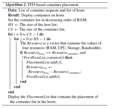
Deploy the PlacementList that contains the placement of the container list in the hosts;

3.2. Forecasting Energy Consumption

To predict the energy consumption in the data centers, we will calculate the energy consumed by the system of active hosts and storage. This energy will help us predict the energy consumed by other equipment such as the cooling system. The following figure shows the distribution of energy consumed by a data center based on studies and previous work.

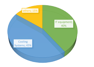
Figure 5: The distribution of energy consumption of a data center

To predict the energy consumed by active hosts, we rely on the placement of containers in these servers. This workload placement will help us determine the percentage used for hardware resources (RAM, CPU, Storage, Bandwidth) of each active host. The calculated percentages will be sorted between 0 (0%) and 1 (100%) to simplify their use in the CloudSim power model. Based on these percentages, we will define for each host the energy consumed by each resource in watts. The following equation represents the energy consumed in watts by a resource according to its percentage of use for a host.

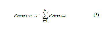
Predicting the energy consumed by each resource will help us to define the energy consumption for a single host and for all active servers that are defined by the following two equations.

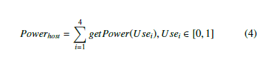
The Use₁ is the used value of the RAM, Use₂ is the used value of CPU, Use₃ is the used value of the BW, and Use₄ is the used value of the Storage.

We represent below our algorithm for predicting the energy consumed by a data center based on container placement.

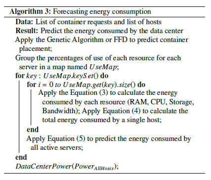
Apply Equation (5) to predict the energy consumed by all active servers; end DataCenterPower(Power_AllHosts);

So, to predict the total energy consumed by a data center, we will rely on the energy predicted for the active host system. Algorithm (3) predicts the energy consumed by the active hosts in the data center based on the placement of workloads. Based on Figure 5 and previous work, we noted that the energy consumption of a data center is divided into three classes. The cooling system takes a large proportion with a value between 45% and 50% (47% on average). For the active host system and storage equipment, their consumption is between 36% and 40% (38% on average). Other systems such as lighting and communication equipment consume 15% of the total energy.

4. Experiments and Results

To evaluate our approach, we used CloudSim 4.0 to apply our algorithms to homogeneous and heterogeneous cloud systems. Our experiments will present the prediction of container placement, then the energy consumption for each system. In this section, we will perform three different experiments. In the first two applications, we will have two scenarios.

4.1. Application 1 : Homogeneous System

The homogeneous system we used in this experiment consists of 50 identical servers in terms of material resources and 3000 containers of different classes.

Table 1: Details of the Application 1

System	Number	RAM (MB)	Number of CPUs	Bandwidth	Storage (MB)
Hosts	50	65536	512	2000000	2000000
Containers (class 1)	1000	512	1	2500	1024
Containers (class 2)	1000	256	1	2500	1024
Containers (class 3)	1000	128	1	2500	1024

4.1.1 SCENARIO 1 : When all hosts are active and the percentage of use of each resource = 50%

In this scenario, we decided to predict the energy consumed by this data center in the case where the use of each material resource equals 50%. The following table shows the results obtained in detail.

Table 2: Energy consumption for the scenario 1 of Application 1

             RAM use                            CPU use                       Bandwidth use                 Storage use

              (watts)                               (watts)                               (watts)                            (watts)

5800	5800	5800	5800
	Number of active hosts : 50
Energy consumption of active hosts (38%)	Energy consumption of cooling system (47%)	Energy consumption of others (15%)	Energy consumption of the data center

          23200.0 watts                 28694.736 watts                9157.895 watts              61052.63 watts

4.1.2. SCENARIO 2 : Genetic Algorithm application

This scenario represents the application of our genetic algorithm for the prediction of container placement and the energy consumption of the different systems of the data center. The results obtained are as follows.

Table 3: Energy consumption for the scenario 2 of Application 1

             RAM use                            CPU use                       Bandwidth use                 Storage use

              (watts)                               (watts)                               (watts)                            (watts)

2288.932	1920.636	1828.676	1738.72
	Number of active hosts : 18
Energy consumption of active hosts (38%)	Energy consumption of cooling system (47%)	Energy consumption of others (15%)	Energy consumption of the data center

          7776.964 watts                 9618.877 watts                3069.8542 watts            20465.693 watts

4.1.3. SCENARIO 3 : FFD application

In this scenario, we applied the First-Fit Decreasing algorithm to place the container list and predict the energy consumed by this data center after completing the workload placement. The following table shows the results obtained.

Table 4: Energy consumption for the scenario 3 of Application 1

             RAM use                            CPU use                       Bandwidth use                 Storage use

              (watts)                               (watts)                               (watts)                            (watts)

2288.932	1826.91	1830.826	1739.208
	Number of active hosts : 18
Energy consumption of active hosts (38%)	Energy consumption of cooling system (47%)	Energy consumption of others (15%)	Energy consumption of the data center

          7782.606 watts                9625.8545 watts               3072.0813 watts            20480.543 watts

The objective of the first scenario is to see the rate of energy that will be consumed if a data center hosts a given workload but without any strategy to define its conception so as not to fall into the problem of waste of resources which implies an expansion of energy consumption. In this scenario, each host consumed 464 watts because they are identical. The fact that the 50 hosts are all active, involved an expansion of the total energy consumed that exceeded 61052 watts, which is ordinary because all servers are active. This scenario shows the importance of defining a strategy for the placement of data center workloads and seeing the impact when a strategy is applied to place containers in an minimal number of servers. The application of the genetic algorithm gave two solutions of 18 servers for each that will be active to host the 3000 containers. We noticed in each solution that the power consumption of the hosts is close to each other (between 400 and 476 watts). As well as workloads are well distributed among active servers (a good load balancing). For total energy consumption, the first solution predicted a value of 20465.693 watts with 40586.937 saved energy compared to the first scenario. The second solution estimates the energy consumption with 20466.234 watts and 40586.396 watts of energy saved when compared with the solution of scenario 1.

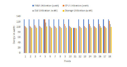
Figure 6: The energy consumed in watts by each resource for the GA first solution Application 1

Like the genetic algorithm, the FFD proposed a single arrangement of 18 hosts among the starting 50 to place the list of containers. So, 32 will be retained, contrary to the first scenario. Of the 18 active servers, 9 hosts each consumed more than 423 watts, 8 others consumed between 427 and 476 watts for each, and only one server that is the last one consumed less than 400 watts (383.59146 watts). The placement proposed by the FFD also gave good results for the total energy consumption (20480.543 watts) which is lower than in the first scenario with a value of 40572.087 watts of energy saved. But the solutions of the genetic algorithm are better in terms of the energy consumed but identical to that of the FFD in the number of active hosts.

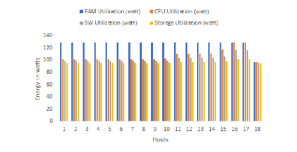
Figure 7: The energy consumed in watts by each resource for the FFD solution Application 1

4.2. Application 2 : Heterogeneous System

In this application, we used a heterogeneous system that consists of three different types of hosts with a total number of 50, and 3000 containers.

Table 5: Details of the Application 2

System	Number	RAM (MB)	Number of CPUs	Bandwidth	Storage (MB)
Hosts (class 1)	17	32768	256	2000000	2000000
Hosts (class 2)	17	65536	512	2000000	2000000
Hosts (class 3)	16	131072	640	2000000	2000000
Containers (class 1)	1000	512	1	2500	1024
Containers (class 2)	1000	256	1	2500	1024
Containers (class 3)	1000	128	1	2500	1024

4.2.1. SCENARIO 1 :

When all hosts are active and the percentage of use of each resource = 50%

In the first scenario of application 2, we predicted the energy consumed for a heterogeneous system when all servers are active.

Table 6: Energy consumption for the scenario 1 of Application 2

             RAM use                            CPU use                       Bandwidth use                 Storage use

              (watts)                               (watts)                               (watts)                            (watts)

6202	6202	6202	6202
	Number of active hosts : 50
Energy consumption of active hosts (38%)	Energy consumption of cooling system (47%)	Energy consumption of others (15%)	Energy consumption of the data center

          24808.0 watts                 30683.578 watts                9792.632 watts              65284.21 watts

4.2.2. SCENARIO 2 : Genetic Algorithm application

Scenario 2 represents the application of the genetic algorithm on our heterogeneous system. The results are as follows.

Table 7: Energy consumption for the scenario 2 of Application 1

             RAM use                            CPU use                       Bandwidth use                 Storage use

              (watts)                               (watts)                               (watts)                            (watts)

1944.637	1594.332	1450.27	1193.698
	Number of active hosts : 11
Energy consumption of active hosts (38%)	Energy consumption of cooling system (47%)	Energy consumption of others (15%)	Energy consumption of the data center

          6182.937 watts                7647.3164 watts                2440.633 watts             16270.887 watts

4.2.3. SCENARIO 3 : FFD application

For this scenario, we applied the FFD algorithm. Below is the prediction of the energy consumed by our system after this application.

Table 8: Energy consumption for the scenario 3 of Application 2

              RAM use                            CPU use                       Bandwidth use                 Storage use

               (watts)                               (watts)                               (watts)                            (watts)

3049.891	2592.923	2448.035	2358.184
	Number of active hosts : 26
Energy consumption of active hosts (38%)	Energy consumption of cooling system (47%)	Energy consumption of others (15%)	Energy consumption of the data center

          10449.033 watts               12923.805 watts               4124.6187 watts            27497.457 watts

In the second application, we used a heterogeneous system to see if the placement of the containers and the rate of energy consumption will be influenced by the nature of the system. In the first scenario, the 50 hosts consumed a different energy rate because they are heterogeneous. The first 17 servers consumed 408 watts each, and the last 16 consumed the high value (624 watts each). The other servers consumed 464 watts each. For the total energy consumption, the system consumed 65284.21 watts with superiority of 4231.58 compared to scenario 1 of the first application.

The application of the genetic algorithm for this heterogeneous system gave two different solutions in contrast to scenario 2 of Experiment 1 which proposed two identical solutions at the level of the proposed number of active hosts. The heterogeneous nature of this system has increased the chance of having diversified solutions in terms of the hosts used and their number.

The first solution obtained by the genetic algorithm has proposed 13 servers that will be active to host the container list, which is the best number compared to the first scenario. The energy consumption of the 13 active servers is between 350 and 800 watts because of the hosts’ diversity in the hardware resources. This diversity influenced the rate of energy consumed by the data center which did not exceed 17623.83 watts with 47660.38 watts of energy saved compared to scenario 1.

The second solution was the best with 11 active hosts and less than 2 servers compared to the first solution to host workloads. The values consumed of energies differ from one host to another because of the diversity in material resources. This number of active servers influenced the energy consumption rate, which was minimized at the level of all the data center systems and 1352.943 watts for the total consumption.

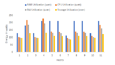
Figure 8: The energy consumed in watts by each resource for the GA second solution – Application 2

The unique solution of the FFD is different from those of the genetic algorithm. The solution offers 26 servers for container placement which is not optimal when compared with the solutions of scenario 2. This increase in the number of active hosts for the FFD is because of its way of assigning containers to servers which is classic and avoids waste of space but is not always effective if there is a list of containers in a defined order (increasing or decreasing). For this reason, most of the active hosts (17) belong to class 1 and the others belong to the second class.

So workloads were not well distributed between the active hosts about the solution of the genetic algorithm, which is a weak point in the FFD algorithm. The high number of active servers consumed between 370 and 480 watts for each, implied an increase in the rate of energy consumed by the data center with a value of 27497.457 watts.

We note that the genetic algorithm guarantees best container placement and minimal energy consumption due to its functioning which is adaptive to different types of systems. But in general, both algorithms offer a good solution for virtualization in a data center, which is important for the whole system to operate without any waste of resources that can increase energy consumption

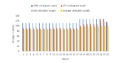
Figure 9: The energy consumed in watts by each resource for the FFD solution -Application 2

4.3. Application 3 : Global Comparison

After testing our algorithms, we decided to compare them with other previous heuristic or meta-heuristic methods to properly evaluate our algorithms. For this, we chose the approach in [19] which uses the Simulated Annealing (SA) algorithm to predict the placement of virtual machines based on the estimate of energy consumption to choose the best placement. In our case, we will evaluate this algorithm using container instances to compare it with our genetic algorithm (GA). More of this we will compare the approach proposed in [33] which applies the Ant Colony Optimization (ACO) for container placement with our genetic algorithm (GA).

The choice of the Simulated Annealing and ACO to examine the effectiveness of our genetic algorithm was not random, but due to several reasons. First of all these three algorithms belong to the class of metaheuristics which is inspired by nature to solve optimization problems. More of that, they can adapt to problems with a high complexity and which require a huge calculation. Another point that encouraged us more to compare our Genetic Algorithm with Simulated Annealing and the ACO is that the works [19] and [33] have the same vision regarding the placement of virtual instances by optimizing the use of material resources and uses the same procedure, except that the work [19] are based on virtual machines instead of containers. For the FFD, we will evaluate it with First-Fit (FF) and Random-Fit (RF) which are algorithms of the Bin Packing problem such as the FFD. Table 9 shows the resources of the different cloud systems used on which we will perform our comparison.

Table 10 represents the results obtained for the energy consumption of several data centers for each algorithm.

Table 10 represents three main results for six algorithms. For each system, we applied six algorithms to predict the energy consumed by each data center based on container placement. As well as, we calculated the energy saved or conserved for each system by comparing the predicted energy consumption with the energy consumed when all the hosts of a system are active and the percentage of use of each resource = 50%. In addition, we calculated the execution time of each algorithm.

For the first system which is homogeneous, we notice that the energy consumption obtained by the genetic algorithm does not exceed 13460 watts with 47594.73 watts of saved energy. For the ACO algorithm, the energy consumption exceeded the value predicted by the genetic algorithm twice with 32931.009 watts of stored energy. Similarly, for the SA algorithm, the energy consumed exceeded that of GA but with a big difference which influenced the rate of energy saved which was less than 10380 watts. On the other hand, the execution time of the genetic algorithm was very high (more than 31 seconds) compared to that of ACO which gave its result in 0.297 seconds and the SA in 5.62 seconds. The reason why the execution time of the genetic algorithm is very high is because of its execution process that operates under several iterations (in our case 100 iterations).

For heuristics, the three Bin Packing problem-solving algorithms (FFD, FF, and RF) predicted energy consumption values close to each other. The values proposed by the FFD and FF were identical to the superiority of the RF algorithm which gave a value of 13447.468 watts which is optimal compared to those of the FFD and FF. For the energy saved, the three heuristics provided better values with the genetic algorithm, but they are fast in execution time because they produce a single solution without using several iterations.

In the second system, which is heterogeneous, the results obtained by the genetic algorithm for the energy consumed and saved are the best when compared with those of ACO and SA and also with the three heuristics. On the other hand, its execution time which reached 31 seconds is very high compared to the other algorithms. We also notice that the FFD, FF, and RF gave the same energy consumption value (31874.584 watts), but the RF surpasses them in the execution time (0.08 seconds). The same goes for the third system, which has a superiority of the genetic algorithm over the others in terms of the energy consumed which is optimal, but the execution time has increased greatly (301.769 seconds) because of the size of the number of instances in this system. The SA also took 103.123 seconds which is high compared to other methods.

Table 9: Details of the Application 3 Hosts Containers System Number RAM (GB) Number of CPUs Bandwidth Storage (MB) Number RAM (MB) Number of CPUs Bandwidth Storage (MB) 1 50 32 256 2000000 2000000 334 512 1 1024 2500 334 256 1 1024 2500 332 128 1 1024 2500 2 17 16 128 2000000 2000000 1000 512 1 1024 2500 17 32 256 2000000 2000000 16 64 512 2000000 2000000 3 25 16 128 2000000 2000000 667 128 1 1024 2500 25 32 256 2000000 2000000 667 256 1 1024 2500 25 64 512 2000000 2000000 666 512 1 1024 2500 4 100 64 512 2000000 2000000 1667 512 1 1024 2500 1667 256 1 1024 2500 1666 128 1 1024 2500 5 34 32 256 2000000 2000000 1667 128 1 1024 2500 34 64 512 2000000 2000000 1667 256 1 1024 2500 32 128 1024 2000000 2000000 1666 512 1 1024 2500 6 30 256 1024 4000000 4000000 3500 256 1 1024 2500 30 128 1024 4000000 4000000 30 64 512 4000000 4000000 3500 512 1 1024 2500 30 32 256 4000000 4000000 Table 10: Comparison of different algorithms for predicting the energy consumption of different cloud systems GA ACO SA System Data Center Energy (watt) Energy Saved (watt) Execution time (second) Data Center Energy (watt) Energy Saved (watt) Execution time (second) Data Center Energy (watt) Energy Saved (watt) Execution time (second) 1 13457.9 47594.73 31.954 28121.621 32931.009 0.297 50678.336 10374.294 5.62 2 18792.02 42260.61 31.004 39339.375 21713.255 0.179 51927.41 9125.22 4.034 3 20413.207 71165.743 301.769 53369.266 38209.684 0.264 77419.08 14159.87 103.123 4 43210.434 121000.086 5304.5 67590.805 96619.715 1.496 100156.78 64053.74 3870.694 5 28867.098 101701.322 3886.164 77247.85 53320.57 1.17 98288.49 32279..93 1165.504 6 19218.874 148149.546 11634.408 31827.826 135540.594 1.126 116079.95 51288.47 1317.876 FFD FF RF System Data Center Energy (watt) Energy Saved (watt) Execution time (second) Data Center Energy (watt) Energy Saved (watt) Execution time (second) Data Center Energy (watt) Energy Saved (watt) Execution time (second) 1 13462.325 47590.305 0.194 13462.325 47590.305 0.122 13447.468 47605.162 0.118 2 31874.584 29178.046 0.116 31874.584 29178.046 0.062 31874.584 29178.046 0.08 3 40164.184 51414.766 0.351 40546.266 51032.684 0.2 40333.258 51245.692 0.287 4 43202.652 121007.868 7.788 43202.652 121007.868 8.441 43329.03 120881.49 2.856 5 48174.152 82394.268 2.93 48301.848 82266.572 2.594 48233.105 82335.315 2.186 6 21229.072 167368.42 12.186 21242.38 146126.04 8.91 21098.488 146269.932 10.894

For other systems, our genetic algorithm was the best in systems 5 and 6 in terms of optimal energy consumption, but it takes a long time to finish its execution and give the final results. In system 4, the FFD and FF heuristics proposed optimal solutions with an energy value of 43202.652 watts which is less than 7782 watts compared to the value proposed by the genetic algorithm. Generally, our GA has proposed best values for energy consumption for most systems ahead of other metaheuristics (ACO and SA) and even heuristics. On the other hand, execution time remains its main weakness because of its way of solving the problem. FFD was best with RF in the heuristics used. In terms of execution time, the ACO was the best with an average time of 0.75 seconds. More of this the SA algorithm proposed large energy values and ranked second before the genetic algorithm at the level of execution time.

5. Conclusion

In this paper, we have presented an approach based on heuristics and metaheuristics for predicting the energy consumed by different data centers based on the placement of workloads. Our approach has proposed a genetic algorithm and a First-Fit Decreasing using cloud containers to predict the best and optimal placement for these instances in several servers without wasting hardware resources. The results obtained showed that the genetic algorithm guarantees a good placement for containers and minimizes the energy consumption in the data centers, after comparing it with other metaheuristics such as Ant Colony Optimization and Simulated Annealing.

Conflict of Interest

The authors declare no conflict of interest.

1. A. Bouaouda, K. Afdel, R. Abounacer, “Forecasting the Energy Consumption of Cloud Data Centers Based on Container Placement with Ant Colony Opti- mization and Bin Packing,” in 2022 5th Conference on Cloud and Internet of Things (CIoT), 150–157, 2022, doi:10.1109/CIoT53061.2022.9766522.
2. A. Greenberg, J. Hamilton, D. A. Maltz, P. Patel, “The Cost of a Cloud: Re- search Problems in Data Center Networks,” SIGCOMM Comput. Commun. Rev., 39(1), 68–73, 2009, doi:10.1145/1496091.1496103.
3. G. Wu, M. Tang, Y.-C. Tian, W. Li, “Energy-Efficient Virtual Machine Place- ment in Data Centers by Genetic Algorithm,” in T. Huang, Z. Zeng, C. Li,
   C. S. Leung, editors, Neural Information Processing, 315–323, Springer Berlin Heidelberg, Berlin, Heidelberg, 2012.
4. A. Mosa, N. Paton, “Optimizing virtual machine placement for energy and SLA in clouds using utility functions,” Journal of Cloud Computing, 5, 2016, doi:10.1186/s13677-016-0067-7.
5. “Cloud Computing Energy Efficiency, Strategic and Tactical Assessment of En- ergy Savings and Carbon Emissions Reduction Opportunities for Data Centers Utilizing SaaS, IaaS, and PaaS,” Technical report, Pike Research, 2010.
6. M. Dayarathna, Y. Wen, R. Fan, “Data Center Energy Consumption Modeling: A Survey,” IEEE Communications Surveys Tutorials, 18(1), 732–794, 2016, doi:10.1109/COMST.2015.2481183.
7. “Energy efficiency policy options for australian and new zealand data centres,” Technical report, The Equipment Energy Efficiency (E3) Program, 2014.
8. R. Brown, E. Masanet, B. Nordman, B. Tschudi, A. Shehabi, J. Stanley, J. Koomey, D. Sartor, P. Chan, J. Loper, S. Capana, B. Hedman, “Report to Congress on Server and Data Center Energy Efficiency: Public Law 109-431,” 2007, doi:10.2172/929723.
9. D. Boru, D. Kliazovich, F. Granelli, P. Bouvry, A. Y. Zomaya, “Energy-efficient data replication in cloud computing datacenters,” in 2013 IEEE Globecom Workshops (GC Wkshps), 446–451, 2013, doi:10.1109/GLOCOMW.2013. 6825028.
10. W. Van Heddeghem, S. Lambert, B. Lannoo, D. Colle, M. Pickavet, P. De- meester, “Trends in worldwide ICT electricity consumption from 2007 to 2012,” Computer Communications, 50, 64–76, 2014, doi:https://doi.org/10. 1016/j.comcom.2014.02.008, green Networking.
11. “Facts & stats: Data architecture and more data,” Technical report, Info-Tech, 2010.
12. Greenpeace, “Make It Green: Cloud Computing and its Contribution to Climate Change,” Technical report, Greenpeace International, 2010.
13. A. Sharma, N. Nitin, “A Multi-Objective Genetic Algorithm for Virtual Ma- chine Placement in Cloud Computing,” International Journal of Innovative Technology and Exploring Engineering (IJITEE), 8, 2278–3075, 2019.
14. G. Dasgupta, A. Sharma, A. Verma, A. Neogi, R. Kothari, “Workload Man- agement for Power Efficiency in Virtualized Data Centers,” Commun. ACM, 54(7), 131–141, 2011, doi:10.1145/1965724.1965752.
15. G. Warkozek, E. Drayer, V. Debusschere, S. Bacha, “A new approach to model energy consumption of servers in data centers,” in 2012 IEEE International Conference on Industrial Technology, 211–216, 2012, doi:10.1109/ICIT.2012.6209940.
16. L. Liu, H. Wang, X. Liu, X. Jin, W. He, Q. Wang, Y. Chen, “GreenCloud: a new architecture for green data center,” 2009, doi:10.1145/1555312.1555319.
17. X. Fan, W.-D. Weber, L. A. Barroso, “Power Provisioning for a Warehouse- Sized Computer,” SIGARCH Comput. Archit. News, 35(2), 13–23, 2007, doi:10.1145/1273440.1250665.
18. D. Meisner, T. F. Wenisch, “Peak power modeling for data center servers with switched-mode power supplies,” in 2010 ACM/IEEE International Sym- posium on Low-Power Electronics and Design (ISLPED), 319–324, 2010, doi:10.1145/1840845.1840911.
19. K. Dubey, S. C. Sharma, A. A. Nasr, “A Simulated Annealing based Energy- Efficient VM Placement Policy in Cloud Computing,” in 2020 International Conference on Emerging Trends in Information Technology and Engineering (ic-ETITE), 1–5, 2020, doi:10.1109/ic-ETITE47903.2020.119.
20. Y. Wu, M. Tang, W. Fraser, “A simulated annealing algorithm for energy efficient virtual machine placement,” in 2012 IEEE International Confer- ence on Systems, Man, and Cybernetics (SMC), 1245–1250, 2012, doi: 10.1109/ICSMC.2012.6377903.
21. J. Xu, J. A. B. Fortes, “Multi-Objective Virtual Machine Placement in Virtu- alized Data Center Environments,” in 2010 IEEE/ACM Int’l Conference on Green Computing and Communications and Int’l Conference on Cyber, Physi- cal and Social Computing, 179–188, 2010, doi:10.1109/GreenCom-CPSCom. 2010.137.
22. Y. Gao, H. Guan, Z. Qi, Y. Hou, L. Liu, “A multi-objective ant colony system algorithm for virtual machine placement in cloud computing,” Jour- nal of Computer and System Sciences, 79(8), 1230–1242, 2013, doi:https://doi.org/10.1016/j.jcss.2013.02.004.
23. S. Pang, W. Zhang, M. Tongmao, Q. Gao, “Ant Colony Optimization Algo- rithm to Dynamic Energy Management in Cloud Data Center,” Mathematical Problems in Engineering, 2017, 1–10, 2017.
24. A. Kansal, F. Zhao, J. Liu, N. Kothari, A. A. Bhattacharya, “Virtual Machine Power Metering and Provisioning,” in Proceedings of the 1st ACM Symposium on Cloud Computing, SoCC ’10, 39–50, Association for Computing Machinery, New York, NY, USA, 2010, doi:10.1145/1807128.1807136.
25. P. Dziurzanski, S. Zhao, M. Przewozniczek, M. Komarnicki, L. S. Indru- siak, “Scalable distributed evolutionary algorithm orchestration using Docker containers,” Journal of Computational Science, 40, 101069, 2020, doi: 10.1016/j.jocs.2019.101069.
26. C. Zaher, “For CTO’s: the no-nonsense way to accelerate your business with containers,” Technical report, Canonical Limited 2017. Ubuntu, Kubuntu, 2017.
27. D. Bernstein, “Containers and Cloud: From LXC to Docker to Kubernetes,” IEEE Cloud Computing, 1(3), 81–84, 2014, doi:10.1109/MCC.2014.51.
28. O. Kramer, Genetic Algorithms, 11–19, Springer International Publishing, Cham, 2017, doi:10.1007/978-3-319-52156-5 2.
29. I. Boussa¨ıd, J. Lepagnot, P. Siarry, “A survey on optimization metaheuris- tics,” Information Sciences, 237, 82–117, 2013, doi:https://doi.org/10.1016/ j.ins.2013.02.041, prediction, Control and Diagnosis using Advanced Neural Computations.
30. N. Janani, R. Jegan, P. Prakash, “Optimization of Virtual Machine Place- ment in Cloud Environment Using Genetic Algorithm,” Research Journal of Applied Sciences, Engineering and Technology, 10, 274–287, 2015, doi: 10.19026/rjaset.10.2488.
31. A. Wolke, B. Tsend-Ayush, C. Pfeiffer, M. Bichler, “More than bin packing: Dynamic resource allocation strategies in cloud data centers,” Information Systems, 52, 83–95, 2015, doi:https://doi.org/10.1016/j.is.2015.03.003, special Issue on Selected Papers from SISAP 2013.
32. R. Panigrahy, K. Talwar, L. Uyeda, U. Wieder, “Heuristics for Vector Bin Packing,” 2011.
33. O. SMIMITE, K. AFDEL, “Hybrid Solution for Container Placement and Load Balancing based on ACO and Bin Packing,” International Journal of Advanced Computer Science and Applications, 11(11), 2020, doi:10.14569/IJACSA.2020.0111174.

(Click Here)