1. Introduction

Programming computers to learn from data is the subfield of artificial intelligence (AI) known as machine learning (ML). In machine learning, support vector machines (SVM) are among the most frequently used classical supervised classification models [1]. The decision boundary and the hyperplane of the data points are divided into two classes by a pair of parallel hyperplanes that are discovered by SVM [2, 3]. However, there is also machine learning at the particle level called quantum computing. Quantum computing is computation using quantum mechanical phenomena such as superposition and entanglement. The difference is from the computer we use today, which is an electronic base on binary state based on transistors. Whereas simple digital computing requires data to be encoded into a binary number where each bit is in a certain state 0 or 1, quantum computing uses quantum bits (qubit). This can be a superposition of state, both 0 and 1 simultaneously. In quantum computing, a new algorithm is required for that problem, i.e., a normal algorithm used in a classical computer cannot be copied and run on a quantum computer at all. The Quantum Computer Algorithm for popular algorithms such as Prime factorization of integers Shor’s algorithm is a quantum algorithm that can attack the algorithm RSA and encryption process of 90% of computer systems worldwide in a short period. Quantum computers can also operate on qubits using quantum gates and measurements that change the observed state. Quantum gates and problems encode input variables into quantum states. To facilitate further modeling of the quantum state, quantum algorithms often exhibit probabilities in which they provide guidance for valid only for known probabilities. Quantum machine learning (QML) is an emerging interdisciplinary research field that combines quantum physics and machine learning, using it to help optimize and speed up data processing on the quantum state. In addition to the widespread popularity of QML, there is also the variational quantum classifier (VQC) for solving classification problems. At present, IBM has developed a quantum computer open to researchers or anyone interested in using it called IBM Q Experience, with a set of instructions developed in Python called Qiskit, which has a simulated quantum computer and real 5- and 15-qubit quantum computers to develop and test circuits. In this article, we present an experiment, which is a continuation of previous experiments [4, 5], that studied the forecast of water release from the dam and the weather forecast behind Pa Sak Jolasid Dam, respectively. Both experiments used a classical machine learning process that measures all model results as model accuracy. The model results are satisfactory.”

In this paper, an experiment was performed using a Quantum Machine Learning classifier and applying it to real data, which brought information from the weather station located behind the Pa Sak Jonlasit Dam. The Pa Sak Jolasid Dam is an earth dam with a clay core, 4,860 meters long, and 31.50 meters high. The maximum storage water level is +43.00 MSL, and the water storage capacity is 960 million cubic meters. The total operational budget is 19,230.7900 million baht, and the satellite coordinates are n14.964687, e101.022677 (see Fig.1). The red dot on the map represents the location of the weather station. Studying weather conditions, especially forecasting rainy days, can benefit water inflow management from quantum machine learning classifier techniques applied to actual weather data from Table 1. The total number of data is 1743 samples, divided into 1220 samples of training data and 523 samples of testing data. The number of features has 4 samples or 4 input qubits, and the label has 2 classes. Table 2 shows a sampling of the values of the features, which are average wind, average temperature, average pressure, average humidity, and label values.

A systematic study of the classical feature and optimizer with the different iterations of the parametrized circuits is presented. The study of the weather behind the dam is based on weather data from 2016 to 2022 as a training dataset. Classification is one problem that can be effectively solved with quantum gates. There are several types of classifiers in the quantum domain, such as Quantum Support Vector Machine (QSVM) with kernel approximation, Quantum Neural Networks (QNN), and Variable Quantum Classification (VQC). According to the experiment, Quantum Support Vector Machine (QSVM), Quantum Neural Network (QNN), and Variable Quantum Classification (VQC) achieved 90% accuracy. All of these algorithms were performed using Qiskit, an open-source software development kit (SDK) developed by IBM.

The classification is one problem that can be effectively solved with quantum gates. There are several types of classifiers in the quantum domain such as Quantum Support Vector Machine (QSVM) with kernel approximation [6-8], Quantum Neural Networks (QNN) [9, 10], and Variable Quantum Classification (VQC) [11-14]. The experimental results proved that we can use QML to solve real-world problems that are classically trained and tested before encoding the feature map, evaluating the model, and optimizing it from the algorithm above.

In this article, we will discuss the origin of the theory of quantum applied in section 2, followed by the steps and methods in section 3. Section 4 discusses the experimental results and explains the reasoning. Finally, section 5 provides a summary of the experiments and recommendations.

Regarding the experiment, we applied Quantum Machine Learning classifiers to real data from the weather station located behind the Pa Sak Jolasid Dam. This earth dam has a clay core, and it is 4,860 meters long and 31.50 meters high, with a maximum storage water level of +43.00 MSL, and a water storage capacity of 960 million cubic meters. The total operational budget is 19,230.7900 million baht, with satellite coordinates: n14.964687, e101.022677 (see Fig.1). The red dot on the map represents the location of the weather station, which studies weather conditions, especially forecasting rainy days, and can benefit water inflow management from quantum machine learning classifier techniques applied to actual weather data from Table 1.

The total number of data is 1743 samples, divided into 1220 samples of training data and 523 samples of testing data. The number of features has 4 samples or 4 input Qubits, and the label has 2 classes. Table 2 shows a sampling of the values of the features, which are average wind, average temperature, average pressure, average humidity, and label values. We present a systematic study of the classical feature and optimizer with the different iterations of the parametrized circuits.

In conclusion, the experimental results demonstrate that QML can be used to solve real-world problems, which are classically trained and tested before encoding the feature map, evaluating the model, and optimizing it from the algorithm above. Therefore, the potential applications of quantum machine learning classifiers are promising, and more research in this area should be encouraged

2. Related work

Since we have the weather dataset for the dam, we can make predictions based on the training data. This is a binary classification problem with an input vector x and binary output y in {0, 1}. The goal is to build a quantum circuit that produces a quantum state based on the following study.

2.1.  Quantum Computing

What exactly is a quantum computer then? In a nutshell, it could be described as a physical implementation of n qubits with precise state evolution control. A quantum algorithm, according to this definition of quantum computers, is a controlled manipulation of a quantum system followed by a measurement to obtain information from the system. This basically means that a quantum computer can be thought of as a special kind of sampling device. However, because it is a quantum state, the configurations of the experiments are very important. Any quantum evolution can be approximated by a series of elementary manipulations, known as quantum gates, according to a theorem in quantum information [15]. Quantum circuits of these quantum gates are the basis for many quantum algorithms. The idea of a qubit came from upgrading classical bits [16, 17], which are 0 or 1, to a quantum state.

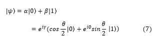
However, what are qubits? Because it is a two-level system defined on , a qubit is frequently referred to as the simplest possible quantum system. This state can be formulated as with  (α, β) and |α|² + |β|² = 1, where  and are hardware-defined orthonormal states known as computational basis states. The qubit is significant because it is in a superposition—that is, it is a either  or  at the same time—which means that, in contrast to classical bits, it possesses a mixture of both. Using tensor products, we can generalize this to include n untangled qubits.

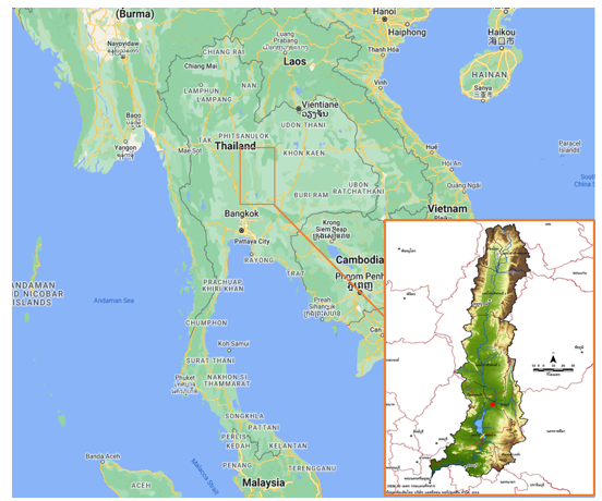
Figure 1: Pa Sak Jolasid Dam, Coordinates: n14.964687, e101.022677.

Table 1. Dataset Attributions Datasets Number of Class Number of Features Train Size Test Size Total Size Weather behind Dam 2 4 1220 523 1743   Table 2. Partial Dataset Date Avg. Wind Avg. Temp Avg. Pressure Avg. Humid Rainfall 2016/10/14 2.3 28 999.4 46 Yes 2017/01/04 6.6 26 1003.7 64 No 2018/03/07 3.3 25.9 1002.8 27 Yes 2019/08/01 3.9 25.4 998.4 86 Yes 2020/10/11 3.4 27.8 999.3 73 Yes 2021/02/22 2.1 26.9 1003.2 48 No 2022/05/12 2.7 28 1000.5 82 Yes

where  stands for qubits. However, the state   would no longer be separable if the qubits were entangled, and every qubit would either be  or , resulting in

with ∈ , and  = 1. Wherever we use the abbreviated notation  := . To make the notation more elegant, we see that the basis states can be written as follows: ↔ ,…, ↔  giving us the straightforward equation. This allows us to translate the notation from binary numbers to integers.

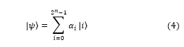
As a result, {|0⟩ …, |i⟩} and n serve as the computational foundation for n qubits. Since there are 2ⁿ distinct strings, one requires 2ⁿ amplitudes  to describe the state of n qubits, as we can see. In other words, quantum information is “larger” than classical information because the information stored in a quantum state with n qubits is exponential in n, whereas classical information is linear in n. which suggests quantum advancements thus far.

2.2.  Quantum Circuit

       We must begin by examining quantum gates in order to construct a quantum algorithm or quantum circuit [18, 19, 20], as mentioned earlier. Unitary transformations are the means by which quantum gates, or rather quantum logic gates, are produced. A straightforward transformation can serve as a quick reminder of what this means.

where  and  are two vector spaces in which U is a unitary operator. By “unitary,” mean that the hermitian conjugate of the operator is the inverse, U^† = U^-1, and that the operator is linear. This is important because we can use it to, for example, display

where, if  is normalized, then by construction it is .

2.2.1 A single Qubit

If we return to the subject of quantum gates, equation (1), the state would either be in the state , which has a probability of |α|²  or in the state , which has a probability of |β|². Formally,  2 x 2 unitary transformations are used to describe single-qubit gates. We can begin by considering the X gate, which functions as the quantum equivalent of the classical NOT gate.

and the reverse This matrix is easily identifiable as one of the Pauli matrices, which are unitary by definition. As a result, we know that we can have at least X, Y, and Z gates with the unitary operators Pauli matrices.

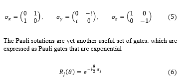
where j is (x, y, z). Since the global phase ( ),  the azimuthal ( ) and polar ( ) angles can be written into any quantum state,

2.2.2 Multi Qubit

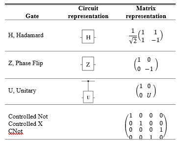
The controlled U gate is introduced because that work on multiple qubits simultaneously. where U can be any unitary gate with one qubit. For instance, the CNOT gate is obtained by setting U = x, and the NOT (X) operation is carried out when the first qubit is in state ; otherwise, nothing changes in the first qubit. A variety of quantum gates, their circuit, and how they are represented in a matrix show table 3. In a controlled gate, the U is a general unitary operator. We refer to j as (x, y, z) and    denotes the appropriate Pauli matrix Eq. (5)

Table 3. Summary of all the gates in circuit and matrix representation.

2.3.  Validation and Measurement

The measurement process is the final step in the theory for quantum computers regarding the quantum circuits that make up a quantum evolution [20]. From quantum mechanics, projectors of the Eigen spaces provide the probability of measuring a state. The probability of measuring i = {0, 1} is

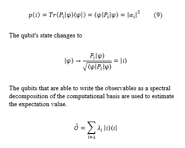
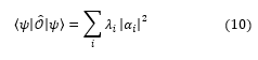
The qubits that are able to write the observables as a spectral decomposition of the computational basis are used to estimate the expectation value.

where P_i is present. Using a Z gate, the observable yields an eigenvalue of +1 for state  and -1 for state  so that we can computationally determine which state it is in (9).

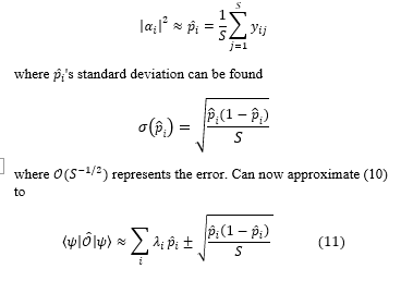
Since all that is required to determine the eigenvalues,  is an estimation of the state’s amplitudes. Since statistics can be used to measure states’ amplitudes directly. They introduce a random Bernoulli variable called y_ij, where P(y_ij = 0) = 1 –  and  P(y_ij = 1) =  [21]. If repeatedly prepare the state  and measure it in the computational basis and collect S samples (y_i1, …, y_iS), additionally, be aware that the frequents estimator can estimate  by

2.4.  Quantum Support Vector Machine (QSVM)

To efficiently compute kernel inputs, the quantum support vector machine QSVM and the quantum kernel estimator (QSVM-Kernel) [20, 22] make use of the quantum state space as a feature space. By applying a quantum circuit  to the initial state , this algorithm nonlinearly maps the classical data x to the quantum state of n qubits:

The 2ⁿ-dimensional feature space created by the quantum circuit  (where n is the number of qubits) is challenging to classically estimate. There are two consecutive layers in this circuit.

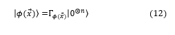
Where  is a unitary operator that encodes the traditional input data, and H is a Hadamard gate Fig. 2.

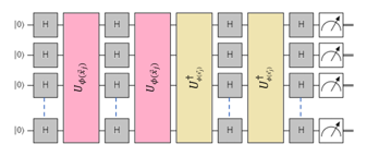
Figure 2. The Circuit of QSVM

During the training phase, the kernel entries are evaluated for the training data and used to locate a separation hyperplane. After that, during the test phase, the new data x and the training data, which are used to classify the new data x according to the separation hyperplane, are used to evaluate the kernel inputs. Quantum computers evaluate the kernel inputs, while classical computers, like those used in a traditional SVM, are used for data classification and separation hyperplane optimization.

2.5.  Variational Quantum Circuit

A variational circuit with four features is proposed in [22] to classify the dataset Fig. 3. The variational circuit performs the following operations. The  state is used to initialize the circuit’s four qubits. The qubits are then placed in a superposition of  and  by applying the Hadamard gate one at a time. Then, a unitary square matrix designed for state preparation is used to perform a unitary operation on each qubit. The classical data (bits) are encoded into qubits in this method.

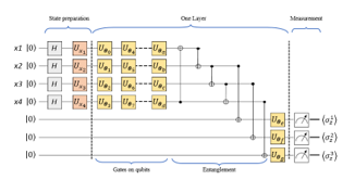
Figure 3. Variational Quantum Circuit

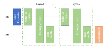
Figure 4. The Variational Quantum Circuit Architecture

Using multiple layers of interleaved rotational gates in data and auxiliary qubits, the variational circuit is designed following state preparation. Optimization is used to adjust the parameters.  Fig. 4. shows the seven-layer initial implementation of the circuit as well as the architecture of the variational circuit model. The class label is obtained by processing the resulting qubits and measuring the auxiliary qubits.

2.6.  Quantum Amplitude Estimation (QAE)

In [20, 23], a hybrid quantum autoencoder (HQA) variant of the Quantum Amplitude Estimation (QAE) algorithm was proposed [24, 25]. Quantum neural networks (QNNs) based on parameterized quantum circuits (PQC) were utilized in this model, which incorporates both classical and quantum machine learning. The model’s overall structure consists of an encoder and a subset of real vector space V of dimension v = dim(V), that transports a quantum state from Hilbert space , as well as a decoder that does the opposite of that. The encoder and decoder’s functional forms are specified, but the models themselves are not specified. As depicted in Fig. 5, the € encoder is a vector α controlled quantum circuit. The circuit applies the unitary U₁(α) after receiving some  states. On the system that combines the input state (v-n) with auxiliary qubits.

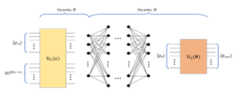
Figure 5. The Quantum Amplitude Estimation Architecture

3.  Methodology

The weather dataset from the Thai Meteorological Department was used as the comparative dataset in the research. The dataset consists of 1773 data sets collected from 2016 to 2022, with 1220 of them being designated for training and 523 for testing. The data is divided into 4 variables for the features and 2 classes for the labels, as shown in Tables 2 and 3. However, there is a fairly standard approach to preprocessing. These strategies are not generally reasonable for planning adequate information for quantum classifiers while working with genuine informational collections. It has proposed a preprocessing strategy in this study, as depicted in Fig. 6, which encrypts the data before the QML algorithm uses it. Two QML classifiers are used in this article:

• A quantum support vector machine
• Build a quantum neural network (also known as Variational Classifier)

Both of the QML classifiers utilized preparation of feature maps, implementation of variational circuits, and measurement. The study analyzed the optimizer’s feature map, the depth of the variational circuit [26], and the depth of the feature map to understand why these models perform optimally, and attempted to determine if the new information can be effectively condensed.

We have using the Qiskit framework for quantum computing. A typical quantum machine learning model consists of two parts, as shown in Fig. 6, A classical part for pre- and post-processing data and a quantum part for leveraging the power of quantum mechanics to simplify certain calculations.

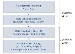
Figure 6: Experimental procedures

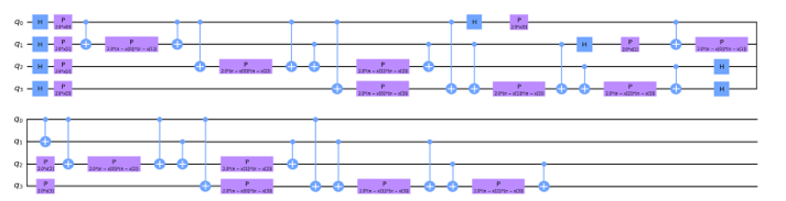
Figure 7: QSVM Featuremaps depths (2).

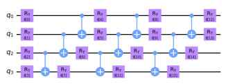
Figure 8: QSVM RealAmplitudes Variational circuit depths (3).

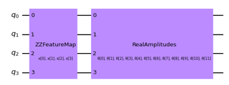
Figure 9: QNN Featuremaps and RealAmplitudes Variational

This study’s experimental design is depicted in Fig. 7. The challenge of training very complex machine learning models on large data sets is one reason for utilizing quantum machine learning.

3.1.  Data preparing and normalization

We shuffle the data to ensure randomness, remove less relevant features, and normalize the information between the ranges of 0 and 2π, and 0 and 1 to properly use the Hilbert space. The data is divided into a training set for model building and a testset for model testing, with the testset size being kept at 30% of the total dataset. This is a common practice in traditional machine learning such as neural networks and support vector machines.

3.2.  Data encoding

Data encoding or state preparation in quantum feature mapping is similar to a classical feature map in that it helps translate data into a different space. In the case of quantum feature mapping, the data is translated into quantum states to be input into an algorithm. The result is a quantum circuit where the parameters depend on the input data, which in our case is the classical weather behind the dam.

It’s worth noting that variational quantum circuits are unique in that their parameters can be optimized using classical methods. We utilized two types of feature maps pre-coded in the Qiskit circuit library, namely the ZZFeaturemap and PauliFeaturemap. To evaluate the performance of different models [27, 28], we varied the depths of these feature maps.

3.3.  Variational quantum circuit

The model circuit is constructed using gates that evolve the input state. It is based on unitary operations and depends on external parameters that can be adjusted. Given a prepared state, , the model circuit U(w) maps  it to another vector,

U(w) is comprised of a series of unitary gates.

4. Results & Discussion

In this research, we make use of the ZZFeaturemap and PauliFeaturemap precoded featuremaps from the Qiskit circuit library. To test the effectiveness of the various models, we changed the featuremaps depths (2). We incorporate more entangle-ment into the model and repeat the encoding circuit by increasing the depth of a feature map. After we used our feature map, a classifier may locate a hyperplane to divide the input data, and a quantum computer can evaluate the data in this feature space as Fig.7. Then we utilized the RealAmplitudes variational circuit from Qiskit. By increasing the depth of the variational circuit, more trainable parameters are introduced into the model that show in Fig. 8. The variational Featuremaps and RealAmplitudes reduced form was applied to write the QNN in Fig. 9. In order to determine the experimental target value in each cycle, the objective function value per iteration of the test was shown in Fig. 10, i.e. QSVM gave less objective value than QNN and VQC in Fig. 11 and Fig. 12, respectively.

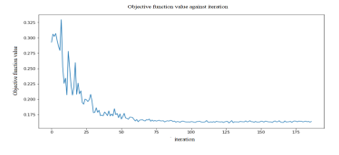
Figure 10: QSVM opjective function value per iteration.

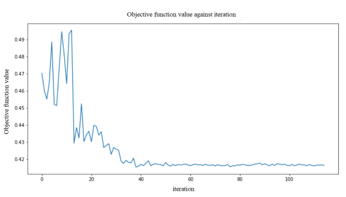
Figure 11: QNN opjective function value per iteration.

Table 4 presents the performance of our models: QSVM, QNN, and VQC. The QSVM obtained an accuracy of 85.3%, while the quantum models QNN and VQC recorded 52.1% and 70.1% accuracy, respectively. The ZZFeaturemap encoding with RealAmplitudes technique was implemented on the model using the weather dataset, with a depth of 3 layers and 300 epochs. The validation accuracy achieved is depicted in Figure 8. Despite the use of three separate attention processes in conjunction with the VQC model, the results of this investigation were satisfactory.

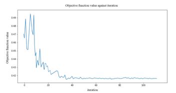
Figure 12: VQC opjective function value per iteration.

Table 4. Classifier test score

Classifier	Score
QSVM	0.853
QNN	0.521
VQC	0.701

5. Conclusion

In this article, we implemented three quantum models using RealAmplitudes techniques. We used ZZFeaturemap encoding as an evaluation optimization, but we acknowledge that this should not be the only optimization used to improve a quantum framework. Furthermore, state preparation is just one aspect of QML algorithms to benefit from when implemented into quantum machine learning. We suggested a pre-processing approach to improve the quantum state preparation for VQC. Our results showed achieved efficiencies of 85.3%, 52.1%, and 70.1%. According to our findings, the QSVM optimizer had the best performance, followed by VQC and QNN. We used ZZFeatureMap with a depth of two and the RealAmplitudes variational form with a depth of three. Moving forward, we plan to explore the use of different data encoding techniques such as RealAmplitudes, amplitude encoding, angle encoding, or other encoding methods to enhance the QML models and increase the number of features to improve performance relative to the established models and cutting-edge techniques. The study was based on a relatively small data set. Therefore, it may influence the assessment of model effectiveness and not discuss data pre-processing techniques because we are primarily interested in the efficiency of quantum models.

Abbreviation

QML                Quantum Machine Learning

QSVM             Quantum Support Vector Machine

QNN                 Quantum Neural Networks

VQC                 Variational Quantum Classifier

SDK                 Software Development Kit

HQA                Hybrid Quantum Autoencoder

QAE                 Quantum Amplitude Estimation

PQC                 Parameterized Quantum Circuits

Conflicts of Interest

The authors declare that there are no conflicts of interest.

Acknowledgements

The authors would like to acknowledge the support from the Computer Engineering Program, College of Innovative Technology and Engineering Dhurakij Pundit University Bangkok, and the support for the information data from the Meteorological Department Thailand.

1. Christopher J.C. Burges A Tutorial on Support Vector Machines for Pattern Recognition Data Mining and Knowledge Discovery volume 2, pages121–167 (1998)
2. Chaiyaporn Khemapatapan and Burada Nothavasi, “Service Oriented Classifying of SMS Message”, 2011 Eighth International Joint Conference on Computer Science and Software Engineering (JCSSE), May 2011, Thailand, pp101-106.
3. Chaiyaporn Khemapatapan, “2-Stage Soft Defending Scheme Against DDOS Attack Over SDN Based On NB and SVM”, Proceeding of 8th International Conference from Scientific Computing to Computational Engineering, Jul 4-7, 2018, Athens Greece, pp.1-8.
4. Thammanoon Thepsena and Chaiyaporn Khemapatapan “Reservoir Release Forecasting by Artificial Neural Network at Pa Sak Jolasid Dam” International STEM Education Conference (iSTEM-Ed 2022), July 6-8, 2022
5. Thammanoon Thepsena, Narongdech Keeratipranon and Chaiyaporn Khemapatapan ” Rainfall Prediction over Pasak Jolasid Dam By Machine Learning Techniques ” National Conference on Wellness Management: Tourism, Technology, and Community (H.E.A.T Congress 2022), August 18-20, 2022
6. Chaiyaporn Khemapatapan, Thammanoon Thepsena and Aomduan Jeamaon “A Classifiers Experimentation with Quantum Machine Lerning” The 2023 International Electrical Engineering Congress (iEECON2023) 2023,
7. Valentin Heyraud, Zejian Li, Zakari Denis, Alexandre Le Boité, and Cristiano Ciuti, “Noisy quantum kernel machines.”, Phys. Rev. A 106, 052421 – Published 18 November 2022
8. Shehab, Omar ; Krunic, Zoran ; Floether, Frederik ; Seegan, George ; Earnest-Noble, Nate, “Quantum kernels for electronic health records classification.”, APS March Meeting 2022, abstract id.S37.006
9. W. Li, Z. Lu and D. Deng1,Quantum neural network classifiers: A tutoria, SciPost Phys. Lect.Notes 61 (2022).
10. S. Laokondee, P. Chongstitvatana, Quantum Neural Network model for Token alloocation for Course Bidding, Computer Science, Physics 2021(ICSEC).
11. Elham Torabian, Roman V. Krems,”Optimal quantum kernels for small data classification.”, Quantum Physics[Submitted on 25 Mar 2022] 14
12. S. Aaronson and A. Ambainis, Forrelation: “A problem that
    optimally separates quantum from classical computing,”, SIAMJ. Comput. 47, 982 (2018).
13. L.Zhou, S.T.Wang, S.Choi, H. Pichler and M.D. Lukin, “Quantum Approximate Optimization Algorithm: Performance, Mechanism, and Implementation on near term device, ” Physical Review X, vol.10, June 2020.
14. E. Farhi, S. Gutmann and J. Goldstone, “A quantum approximate optimization algorithm,”, Nov 2014
15. S. Nath Pushpak, S. Jain, “An Introduction to Quantum Machine Learning Techniques”, 2021 9th Interational conference on Reliability, Infocom Technologies and Optimization, Amity University, Noida, India, 2021
16. Valentin Heyraud, Zejian Li, Zakari Denis, Alexandre Le Boité, and Cristiano Ciuti, “Noisy quantum kernel machines.”, Phys. Rev. A 106, 052421 – Published 18 November 2022, DOI:10.1103/PhysRevA 106.052421
17. Shehab, Omar ; Krunic, Zoran ; Floether, Frederik ; Seegan, George ; Earnest-Noble, Nate, “Quantum kernels for electronic health records classification.”, APS March Meeting 2022, abstract id.S37.006 DOI:10.1109/TQE.2022.3176806
18. W. Li, Z. Lu and D. Deng1,”Quantum neural network classifiers: A tutoria”, SciPost Phys. Lect.Notes 61 2022, DOI: 10.21468/SciPostPhysLectNote.61
19. S.Aaronson and A. Ambainis, Forrelation: “A problem that
    optimally separates quantum from classical computing,” , SIAMJ. Comput. 47, 982 (2018), DOI:10.1137/15M1050902
20. L.Zhou, S.T.Wang, S.Choi, H. Pichler and M.D. Lukin, “Quantum Approximate Optimization Algorithm: Performance, Mechanism, and Implementation on near term device, ” Physical Review X, vol.10, June 2020, DOI:10.1103/PhysRevX.10.021067
21. E. Farhi, S. Gutmann and J. Goldstone, “A quantum approximate optimization algorithm,”, Nov 2014, DOI10.48550/arXiv.1411.4028
22. Maria Schuld and Nathan Killoran “Quantum Machine Learning in Feature Hilbert Spaces.”, Phys. Rev. Lett. 122, 040504 – Published 1 February 2019, DOI:10.1103/PhysRevLett.122.040504
23. Vojtech Havlícek, Antonio D. Córcoles, Kristan Temme, Aram W. Harrow, Abhinav Kandala, Jerry M. Chow & Jay M. Gambetta, “Supervised learning with quantum-enhanced feature spaces.”, Nature volume 567, pages209–212, 2019, DOI:10.1038/s41586-019-0980-2
24. M. L. LaBorde, A. C. Rogers, J. P. Dowling, Finding broken gates in quantum circuits: exploiting hybrid machine learning, Quantum
    Information Processing 19 8,aug 2020, DOI:10.1007/s11128-020-02729-y
25. S. L. Wu, S. Sun, W. Guan, C. Zhou, J. Chan, C. L. Cheng, T. Pham, Y. Qian, A. Z. Wang, R. Zhang, et al. “Application of quantum machine learning using the quantum kernel algorithm on high energy physics analysis at the lhc 2021, DOI:10.1103/PhysRevResearch.3.033221
26. A. Chalumuri, R. Kune, B. S. Manoj, A hybrid classical-quantum approach for multi-class classification, Quantum Information Processing 20, 3 mar 2021, DOI:10.1007/s11128-021-03029-9
27. G. Brassard, P. Høyer, M. Mosca, A. Tapp, Quantum amplitude amplification and estimation, Quantum Computation and Information 2002, P.53–74, DOI:10.1090/conm/305/05215
28. Danyai M., Daniel S., Begonya G. ” Variational Quantum Classifier for Binary Classification: Real vs Synthetic Dataset.” ieee Access. DOI:10.1109/Access.2021.3139323

(Click Here)