1. Introduction

The Latin verb ‘strictus’, which merely means to draw tight, is whence the word “stress” gets its original meaning. The term “stress” didn’t have psychological connotations until the late 19th century, thanks to the groundbreaking work of Hans Selye, who is regarded as the father of stress study. Before then, stress was always thought of as the act of applying physical pressure or force to an object. However, we also experience internal emotional pressures and invisible forces, which has led to a biological investigation into the causes of stress. This was illustrated in the work of W.B. Cannon, who detailed how biological systems have developed an internal system to preserve homeostasis, a stable internal state. In order to test his views concerning acute stress responses as opposed to chronic stress, Hans Selye carried out experiments. He then came up with the phrase “stress responses,” defining stress as pressures or mutual actions that occur across any part of the body, whether it be psychological or physical.

The broad term for stress can be further broken down into two categories: positive stress (Eustress) and negative stress (Distress). Eustress is perceived as a type of pressure that encourages a person to overcome obstacles by learning to see outside pressures as challenges rather than obstacles. On the other hand, distress results from a failure to use these needs as a motivator, which eventually stifles any advancement or success. Distress can also be divided into two categories: acute distress, which is short-term, and chronic distress, which is long-term. It should be highlighted that current definitions and understanding suggest that stress results in a physical reaction as a stressor rather than a physical reaction to perceived threats or challenges.

Both adults and children are afflicted by mental stress. Every human being suffers stress at some point in their lives, whether it is from work-related homework or just plain peer pressure from their employer. Short-term stress may be good for encouraging the improvement of work performed, while long-term stress can be destructive to one’s physical and mental health [1]­. If untreated or without an appropriate management strategy, it can seriously damage cognitive abilities and, as a result, the person’s quality of life [2]. Studies have also revealed that prolonged work stress diminishes the grey matter volumes of the dorsolateral prefrontal cortex and the anterior cingulate cortex, which are accountable for memory, attention, and mood [3].

Despite advances in medicine, particularly in psychology, have made it possible for regular people to get the care or assistance they want. Patients only seek treatment when they can no longer tolerate to live in a situation of extended stress, therefore there is still much to learn and develop in this area. As a result, the general public continues to be untreated and lacks access to expert assistance to lessen future stress. Even worse, because conventional techniques for detecting mental stress primarily depend on self-report questionnaires and interviews, the results are still largely ambiguous. Therefore, subjective interpretations may be used to assess the degree to which a patient’s stress level can be deemed harmful as well as whether or not the patient is experiencing stress. Therefore, the ability to anticipate a patient’s likelihood of experiencing stress in the future or even just identify stress without consulting a medical practitioner may make it possible for patients to receive treatment and possibly even seek it out more voluntarily.

Many attempts have been made up to this point to use a machine learning technique to swiftly evaluate and forecast a patient’s state of health. Results in certain instances point to machine learning’s potential to diagnose conditions more accurately than qualified medical professionals. But in many of these instances, there are numerous flaws and biases, which contribute to the widespread belief that machine learning can supplement, if not completely replace, medical professionals [4]. Nevertheless, we think that machine learning applications in the healthcare industry will only grow. Medical practitioners should then use artificial intelligence and machine learning as a tool to give patients better and more advanced medical care.

By placing tiny electrodes on the scalp, an electroencephalogram (EEG) is a non-invasive, affordable, easily accessible, and painless test that looks for irregularities in brain waves. The potential difference between the cortical neuronal activity and the electrodes’ detection of it is amplified and shown as a waveform. The cortical excitatory and inhibitory postsynaptic potential summations serve as the primary sources of electrographic activity [5]. Additionally, EEG scans reflect changes in brain activity almost instantaneously due to their high temporal resolution, while other scan types require several minutes following the occurrence of an event. Unfortunately, the limited spatial resolution of EEG makes it impossible to pinpoint the precise location of the cerebral waveforms. Furthermore, there will be significant contamination from other electrical noise as a result of the potential difference’s amplification. Even though EEG signals are fascinating, they cannot be used by an interpreter to make future predictions. It’s possible that any waveform anomalies that have happened before won’t happen again.

Based on their frequency range, the waveforms found in an EEG can be grouped. The frequencies at which delta activity, theta activity, alpha activity, beta activity, and gamma activity occur are as follows in increasing order: delta activity occurs between 0.5 and 4 Hz, theta activity between 5 and 7 Hz, alpha activity between 8 and 13 Hz, beta activity between 14 and 30 Hz, and gamma activity between 30 and 80 Hz. Each of these waveforms, in turn, represents distinct brain states, including relaxation, sleep, anxiety, passive attention, and concentration [6]. EEG signal information is a well-known neuroimaging modality that records brain electrical activity for the diagnosis of various brain abnormalities, such as the identification of epileptic seizure activity, depression, stroke, and Alzheimer’s disease [5]. Despite the vast amount of data that can be gleaned from an EEG reading, little research has been done on using it to identify mental stress. Furthermore, the research that has already been done does not consistently point to a general strategy for methodically combining machine learning with EEG for stress assessment [7]. This was demonstrated when various machine learning classifiers and feature extraction techniques were used in comparable circumstances.

Since it has been shown in numerous studies that the alpha, theta, and beta bands of an EEG reading correlate to cognitive workload processing and, in turn, mental stress, here we propose to extract information from these bands in order to classify mental stress [8,9]. Therefore, the purpose of this study is to propose a machine learning (ML) framework for the extraction of EEG features based on fast Fourier transform and wavelet transform for the classification of mental stress, including high- and low-level stress. EEG information from an earlier investigation [10] were decomposed with discrete wavelet transform and fast Fourier transform into different frequency bands, including alpha, theta, and beta, and computed EEG frequency bands power. Widely used ML classifiers, including Support Vector Machine (SVM), Linear Discriminant Analysis (LDA), Decision Trees (DT), and Artificial Neural Networks (ANN), were used to model the EEG dataset in order to illustrate the performance of the suggested ML framework. Next, the Fourier Transform method—a conventional transformation technique for determining power spectral density—is compared to the wavelet transform.

The remaining sections of the paper are organized as section II explains the dataset and feature extraction and classification methodology, section III reports the findings, followed by the discussion in section IV, and finally section V concludes the paper.

2. Literature Review

2.1.  Stress Detection and Appraisal

It’s interesting to note that stress is not a medical diagnosis or condition that calls for medical professionals to thoroughly and methodically evaluate their patients. In actuality, subjective questionnaires like the Perceived Stress Scale (PSS), which has 14 questions (later lowered to 10) that the patient must answer, are the closest measurements of stress that are utilized in a medical setting [11], Stress Response Inventory [11], Holmes and Rahe Stress Scale (Social Readjustment Rating Scale) [12], Depression Anxiety Stress Scale [13], The Hospital Anxiety and Depression Scale [14], The State Trait Anxiety Inventory [15]   and Life Events and Coping Inventory [16].  The PSS was created in 1983 and is still a widely used tool to help us comprehend how various circumstances impact our emotions and our perceived stress levels, which range from low to high. The current problem, however, is that despite all the subjective questionnaires currently in use, the only stress that patients perceive is the stress that they observe and rate for themselves without any concrete data to support the presence or absence of stress. Given that mental stress is the psychological and physiological condition that has afflicted humans for the longest duration, it is unexpected that there isn’t a methodical way to conclusively determine whether stress is present.

Further, doctors and psychologists attempted to use physiological changes mentioned above for an objective measure such as increased heart rate through heart rate variability (HRV) [17]. HRV is where the amount of time between the heartbeats fluctuates slightly usually measured using an electrocardiogram (ECG) that detects the electrical activity of the heart using sensors attached to the skin of the chest. Galvanic Skin Responses (GSR) also known as electrodermal activity (EDA) measures the changes in sweat gland activity that are reflective of the intensity of our emotional state [18]. Moreover, research has tapped into the area of measuring stress through pupil dilation and blood pressure [19]. Consequently, salivary alpha-amylase and cortisol levels were used as a biomarker for stress indication due to their association with the activation of the sympathetic nervous system [20].

2.2.  Electroencephalography

The use of electroencephalography (EEG) to measure stress has been the subject of recent research due to its relative affordability when compared to other methods that involve the collection of blood samples or the ingestion of radioactive chemicals, such as PET scans. But since this method is still relatively new, researchers have had differing degrees of success in identifying stress [5]. Many methods for using EEG signals to detect mental stress have been reported in the literature. These methods include using SVM, Multilayer Perceptron, and Convolutional Neural Networks in a virtual environment to detect mental stress [6]. The detection of stress is still very new and in its early stages, where researchers are still trying to determine electrical signals and patterns related to stress. One drawback of EEG is its limited spatial resolution, which makes it difficult to locate the precise region involved or responsible for stress because the electrical signals measured are only on the surface of the brain. Although there are studies that use direct experimentation and specific regions to identify stress using PET or MRI scans, these approaches are deemed impractical due to the high cost and limited accessibility of the necessary equipment. Furthermore, unlike the other resolution methods mentioned, using an EEG machine does not require extensive training.

2.3.  Machine Learning Methods for Stress Detection

There has been much research that uses artificial intelligence for mental stress assessment through machine learning classifiers and algorithms. A machine learning classifier uses an independent set of information from a dataset known as features to predict the corresponding class it belongs to by having several parameters. Such features need to have unique characteristics that separate one class from another. Further, machine learning classifier will undergo either supervised or unsupervised training to predict the classes of new instances in an unseen testing dataset. Several machine learning techniques and algorithms often used in mental stress assessment are described below.

Machine learning classifiers like SVM, ANN and k-NN have shown immense potential in stress detection with each classifier achieving accuracies of more than 85% [6,21,22]. However, it seems that each classifier is feature specific when comparing each studies above. For example, SVM seems to favor frontal alpha asymmetry as a feature whereas convolutional neural network, a branch of ANN performed much better when simply considering all the brain waves. K-NN on the other hand used only a few selective electrodes and achieved accuracies of 94 and 93.7% [22]. Meanwhile, LDA relied on multiple bio-signals besides EEG such as electrocardiography (ECG), electromyography (EMG) and galvanic skin response (GSR) to perform well [23].

Further, given the complexities of the EEG signals alongside the variability in terms of the experimental conditions, a machine learning end-to-end approach may not be feasible. Among the many limitations of such an approach includes the huge amounts of data that is required to train the classifier alongside the difficulty to validate the output. Therefore, a traditional framework to train each classifier before forming an ensemble is required, especially in domain generalization, nullifying any opportunities to allow for an end-to-end deep learning model to be framed without considering the usual pre-processing and feature extraction process when training a classifier.

It is interesting to note that SVM tops the list of classifiers used when analyzing EEG for stress detection in several review papers [5,24–26]. In fact, SVM is used in almost all the experiments when the Montreal Imaging Stress Task is used as a stressor [24]. This may be because SVM has stronger discriminatory powers than LDA, and less overfitting issues compared to neural networks. However, the field of deep learning for signal processing has been growing lately, especially the usage of pretrained CNN models for robust BCI framework [27].

Recent studies performed also involved the use of SVM classifier alongside Naïve Bayes, and K-Nearest Neighbours (KNN) achieved accuracies of up to 99.98% [28] whereby the participants were induced with stress through the performance of the Stroop Colour Word Test (SCWT). In this study, four different bands were explored, namely the alpha, beta, theta, and delta band before concluding that alpha and beta bands showed a higher accuracy than the other two. Other studies involving the use of K-NN achieved maximum classification accuracy of 91.26% [29]. However, this may be caused by the low number of participants who participated in the study. Another paper involving the use of SVM and Naïve Bayes classifier successfully classified stress and control subjects with up to 98.21% accuracies by focusing on all the power density of the frontal lobes [30]. While both achieved high accuracies in the experiment, it should be noted that these were conducted on subject-wise classification instead of a mixed classification such as control versus mental stress. When dealing with mixed classification, the accuracies dropped to around 80%, a problem that we are trying to address in our study.

2.4.  EEG Wavebands

Alpha waves range from 8 to 12 Hz where it occurs in the occipital head area in the awake state. Regular meditation and relaxation have been shown to enhance alpha waves and the reason for why it is most recommended for lowering stress. Beta waves are most frequently observed around the frontal head zones and most closely associated with stress when there is an increased in beta waves. Delta waves are found in the frontocentral brain area, and these waves are associated with tiredness and early stages of sleep. Theta band is detected in anxiety activation and strongly observed in hypervigilance states such as meditation, prayer, and awareness. Finally, Gamma band is more related to ADHD and knowledge disabilities when there is an inadequate of the activity. Although the Gamma band has been associated with depression when there’s inadequate gamma signals which in turn suggests a relation between mental stress and depression, it remains a relatively unexplored area. There have been multiple findings with regards to the relation of stress and the associated wavebands. Namely the alpha, theta, and beta waves [31,32]. Gamma and Delta bands has been omitted from our experimental design as it has been found that Gamma band is more closely associated to wakefulness than in relation to stress [33]. Whereas Delta band has always been associated with slow brain activity and its occurrence is most prominent during sleep. Nonetheless, some studies have suggested the delta-beta relationship with regards to anxiety [34], a trait that is closely related to mental stress.

3. Materials and Methodology

3.1.  Dataset

Twenty-two healthy individuals (ages 19 to 25) without a history of illness or head trauma make up the EEG dataset. They don’t take any kind of medication that could cause their heart rate to increase. Every participant participated in both the stress and control experimental sessions. They completed the Montreal Imaging Stress Task (MIST)-based Mental Arithmetic Task (MAT) [35] as it has shown the capability of producing stress-related responses involving the hypothalamic pituitary-adrenal (HPA) axis. Accordingly, eight distinct conditions—four stress levels and four control levels—were applied to each participant based on the task’s level of difficulty. Only levels 1 and 4 of stress, along with the controls that go with them, were used in this experiment; level 1 is referred to as low stress, and level 4 as high stress. 128 channels are used to record the EEG data, with a 500 Hz sampling rate. In addition, the other channels are referenced to the 129th channel. Each subject has a total of two sets of 129 channels of EEG data—one for control and one for stress. Prior to being sent to the machine learning classifier for classification, the dataset is normalized. According to the experiment’s original report [10], The EEG trials lasted 2200ms for high stress and control and 1100ms for low stress and control. Therefore, averaged EEG power rather than absolute power is used to compare stress vs. control trials. EEG data from two experimental conditions—low stress versus control condition and high stress versus control condition—were analyzed.

3.2.  EEG Feature Extraction

EEG features are usually divided into three broad categories, the statistical time domain features, frequency domain features, and synchronicity domain features. Statistical time domain features are obtained directly from the raw EEG signals such as calculating the average amplitudes, standard deviation, and variance. Other time domain features frequently used are Hjorth parameters, entropies estimation and Higuchi’s fractal dimension. It should be noted that the raw EEG signals are usually filtered for noise and artefact removal before obtaining any features for machine learning classification. Whereas frequency domain features are usually computed by first converting the raw EEG signals that are in the time domain to the frequency domain alone by applying Fourier transforms or a time-frequency domain via wavelet transforms. Common wavelet transforms usually use Daubechies set of wavelets in the fourth order. In frequency domain features, we can obtain the power spectral density, the distribution of power in its frequency components where power is defined as the amount of energy transferred per unit time, once the raw EEG has been converted. Moreover, absolute and relative powers are commonly used to check the rhythm of EEG signals.

Next, synchronicity domain features use an effective and functional measure of brain connectivity to examine significant coincidences that appear to have no apparent reason. The energy in each frequency is obtained by applying discrete wavelet transforms and Fourier transforms, which are then added to determine the absolute power or averaged to determine the power. With 129 channels and 22 participants from the experimental and control groups, the feature matrix for each EEG frequency band was 44x129x1, yielding a minimum of 5676 (22 x 2 x 129 x 1) features.

3.2.1 Wavelet Transforms

A collection of wave-like oscillations known as wavelets is produced by wavelet transforms, which break down EEG data. Wavelets are a class of functions with a variety of characteristics, including their ability to be stretched to capture high- or low-frequency data; a stretched wavelet will typically capture data at a lower frequency. Furthermore, the function’s integral must have zero mean and finite energy, and its integral squared function must yield a finite number, for a function to be considered a wavelet function. This is how wavelet differs from Fourier analysis, which assumes an infinite integral squared of a sin wave. Subsequently, the wavelet’s location can be adjusted to precisely pinpoint the oscillation point. The wavelet’s location and “stretch-ness” can therefore be changed as we slide it across any given signal. By doing this, the signal input can be represented by the wavelet transforms in both the time and space domains.

Traditionally, the mathematical formula is represented in (1) using the first derivative of a Gaussian function. Increasing the value “a” will stretch the wavelet to capture low frequency information. In contrast, by lowering the value, the parameter “b” establishes the wavelet’s location; a left shift is necessary, and vice versa.

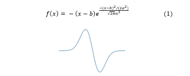
Figure 1: First Gaussian Derivative Function

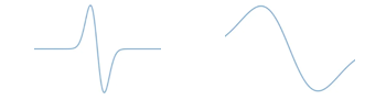
Figure 2: Squishing (left) or Stretching (right) by decreasing or increasing the value of ‘a’

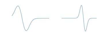
Figure 3: Sliding the gaussian derivative left (left) or right (right) by decreasing or increasing the value of ‘b’

Since a wavelet is made up of a chosen function, such as Gaussian, Harr, Daubechies, and so on, we have chosen to break down the EEG signal into sub-band frequencies using the Daubechies wavelet transform of fourth order (figure 4). This is mostly because, when compared to Haar, Morlet, and other wavelets, an EEG signal’s Daubechies wavelet exhibits striking similarities to it. Moving on, we decompose the signal into 7 levels such that, in each level, half of the signal range is obtained, as shown in figure 1, where A1 to A7 is the approximate coefficient and D1 to D7 is the detailed coefficient. The sampling rate of the EEG data is set at 512 Hz.

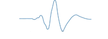
Figure 4:Daubechies Wavelet Function of the fourth order ‘db4’

As a result, we can derive the EEG data’s absolute power within its frequency range. To get the absolute power from all 129 channels, each of the estimated coefficients is squared before being added up. This gives us 129 channels in the alpha, beta, and theta bands, giving us three different sets of features.

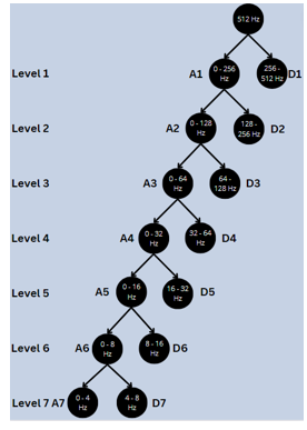
Figure 5: Wavelet Decomposition into 7 Levels

3.2.2 Fourier Transforms

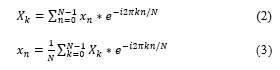
Any given signal can be broken down using Fourier transforms by expanding a periodic function f(x) with an infinite sum of sines and cosines, which is a generalization of the complex Fourier series. It changes the time domain representation of the EEG data to the frequency domain. This is accomplished by using the formula in (2), where N is the number of time samples we have, n is the sample we are currently examining, x_n is the signal’s amplitude at time n, k is the frequency, and X_k is the signal’s amount of frequency k.

We can determine the average power for each frequency band to be used as a feature by averaging the power obtained across the EEG dataset’s sampling rate. Given that Fourier transforms data from the time domain to the frequency domain, it is limited in its applicability to time domain data. As a result, throughout the entire experimental process, we will be unable to determine when exactly the brain region responds to the stressful stimuli.

3.3.  Machine Learning Classifiers

3.3.1 Support Vector Machines

A machine learning classifier called the Support Vector Machine (SVM) looks for a hyperplane in an N-dimensional space, where N is the number of features needed to clearly separate the data points. The SVM will identify the ideal hyperplane by maximizing the margins between two or more data points because there are numerous hyperplanes available to divide data points. In order to construct the position and orientation of the hyperplane, data points that are closest to it are referred to as support vectors.

Since we are only classifying between stress and control classes, the kernel trick method suggested for non-linear dataset was not used. Consequently, MATLAB’s default settings have our SVM’s kernel function set to be linear, and its scale set to “automatic.” The SVM’s box constraint level is set to 1, and its multiclass method is configured as “One vs. One.”.

3.3.2 Linear Discriminant Analysis

Linear Discriminant Analysis (LDA) is an extension of Fisher’s linear discriminant, which looks for a linear feature set that clearly divides two or more classes. The multivariate Gaussian function to be used for prediction is subjected to a calculation of mean and variance when there are multiple feature variables. Plotting the data, however, is assumed by (LDA) to follow the Gaussian function in a bell-curve fashion. It also presumes that the variance around the mean of each feature variable is the same. As a result, the mean, value of each feature variable, x for each class, k, can be calculated by dividing the total number of instances by the sum of values, as shown in the following formula.:

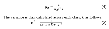
Using the input feature x from equation (6), where  is the prior probability and  is the density function, LDA will apply the Bayes Theorem to estimate the probability of the predicted output class. LDA will use Bayes Theorem to estimate the probability of the predicted output class using the input feature, x that has been given in (6) where is the prior probability and is the density function.

The default implementation of LDA from MATLAB’s classification learner app was used whereby the covariance structure is set as “full”.

 

3.3.3 Decision Tree

A decision tree is conceptualized as a tree root with numerous branches that eventually grow into leaves at the tip. But decision trees are illustrated in reverse, with the root at the top. This means that after applying a starting condition and a given value, the tree may split into branches based on a splitting criterion, ultimately leading to a final output at the leaf. Decision tree splitting criteria are typically based on the ecological diversity index, which provides a quantitative representation of the various species or classes within a dataset.

The Simpson index, on which the Gini’s diversity index is based, gauges the concentration levels when people are categorized into types such that the following probabilities apply when two people are randomly selected from the dataset to represent the same type:

Where  is the total number of classes in the dataset. Gini’s diversity index transforms equation (5) to capture the probability that the two individual data represent different types from the following equation:

MATLAB’s preset for a fine tree to model our decision tree such that the maximum number of splits is set at 100 while the split criterion is based on Gini’s diversity index.

3.3.4 Artificial Neural Network

Artificial neural networks (ANN) are based on the idea of biological neural networks of the brain. Just as a biological neural network consists of the firing of neurons interconnected with synapses, ANN would generally consist of a few layers with connected neurons to simulate the human brain. Mainly, the first layer is known as the input layer as it receives external data as an input. The following layer is the hidden layer that obtains the raw information from the input layer and processes it by applying weights to the inputs and subsequently directs them through an activation function as the output. Finally, the output from the hidden layer is passed to the final layer known as the output layer where the ultimate result such as classifying between stress and non-stress is determined. Most ANNs allow for weight adjustments of the hidden layers by computing the gradient of the loss function with respect to its individual weight. To simplify our experimental set up for neural network models, we decided to use narrow neural network as preset by MATLAB’s built in function whereby there is only one fully connected layer with the first layer size of 10 and the activation function of ReLU.

3.4.  Machine Learning Framework

We extract the absolute and average power features from the collected data using the Fourier and Daubechies wavelet transforms. Next, we’ll feed it into the four machine learning classifiers (SVM, LDA, DT, and NN) that were previously mentioned. Next, the dataset is divided using the ten-fold cross-validation method, which divides the training data into ten distinct subsets, or folds, with 90% of the data in each fold being used for training and the remaining 10% for validation. To get the expected validation accuracy, this is done ten times over. Lastly, ten independent trials are used to train and validate each model to determine the average accuracy, which is displayed in the results section.

4. Experimental Setup, Results and Discussion

MATLAB R2022a was used to develop our machine learning classifiers through the help of the classification learner application using a Windows 10 Operating System running with 8GB RAM and 11th Generation Intel® Core @ 2.40GHz.

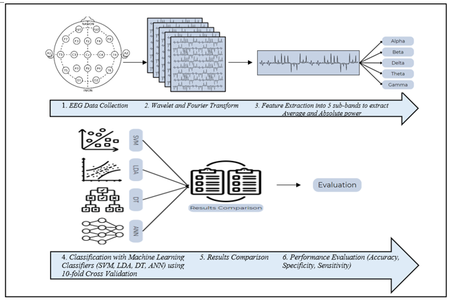
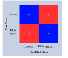
Figure 6a: Sample of Confusion Matrix in Number of Participants

A fair assessment and evaluation are required to determine the usefulness and accuracy of the model. To validate the performance of the model, we have computed the accuracy, sensitivity and specificity of each model using the following equations in (5, 6, 7) based on the confusion matrix from figure 7. True Positive (TP) is used to denote correctly predicted cases while True Negative (TN) is used to denote correctly predicted non-cases. Likewise, False Positive (FP) and False Negative (FN) denotes incorrectly predicted cases and non-cases respectively. A sample of the confusion matrix is shown in figures 7a and 7b respectively where the control group is compared to stress such as low stress or high stress.

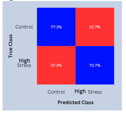
Figure 7b: Sample of Confusion Matrix in Percentages

4.1.  Accuracy

The accuracy of the classifier is denoted by the percentage of true positive (first quadrant) and true negative (fourth quadrant) over the total sum of true positive, true negative, false positive and false negative.

4.2.  Sensitivity

The sensitivity of a classifier is the percentage of correctly predicted cases (True Positives – first quadrant) over the sum of the true positives and false negatives (first and third quadrant).

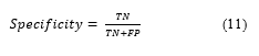
4.3.  Specificity

The specificity of a classifier is the percentage of correctly predicted non-cases (True Negatives – fourth quadrant) over the sum of the true negatives and false positives (fourth and second quadrant).

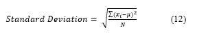
4.4.  Standard Deviation

The standard deviation of each result mentioned is calculated based on formula (12) to indicate the average range of values obtained in 10 trials whereby a small standard deviation value tells us that the accuracy/sensitivity/specificity achieved does not deviate too far from the average value obtained. This is also an indication in our evaluation of whether the classifier performs in a stable manner instead of an erratic manner.

The rest of this section is arranged in the order of the type of machine learning classification used, followed by the experimental conditions of either control vs low stress or control vs high stress and a comparison between low stress vs high stress. Each table shows the result of the averaged validation accuracy, sensitivity, specificity, band spectrum and features used for each classification. Associated alongside is the standard deviation of the model after performing 10 trials. Finally, the best-performing features combination is bolded in each table. Given that absolute power was only used for comparison between stress and control of the same levels, it is not used in different levels as shown in control vs high stress and low stress vs high stress conditions.

Table 1: Support Vector Machine Classifier Results

Support Vector Machine Classification
Control VS Low Stress
Validation Accuracy (%)	Sensitivity (%)		Specificity (%)		Band Spectrum	Features
64.99±2.32	65.79±2.08		60.69±1.21		Alpha	Absolute Power
65.00±3.39	65.62±6.20		58.96±3.29		Theta	Absolute Power
67.05±3.26	72.38±10.42		63.45±5.12		Alpha, Theta	Absolute Power
65.92±3.53	72.79±6.40		63.39±3.16		Alpha, Theta, Beta	Absolute Power
61.14±2.57	55.84±4.77		52.64±2.29		Alpha	Average Power
69.33±2.33	75.68±3.43		65.24±1.79		Theta	Average Power
57.28±3.77	63.92±4.59		58.42±2.77		Alpha, Theta, Beta	Average Power
63.86±2.14	68.54±4.70		62.03±2.76		Alpha, Theta, Beta	Absolute Power, Average Power
Control VS High Stress
82.03±1.24	92.69±2.28	75.13±1.97		Alpha		Average Power
86.83±2.64	94.61±0.23	83.10±2.60		Theta		Average Power
82.88±1.24	91.80±2.68	76.36±2.33		Beta		Average Power
84.10±2.69	94.07±0.16	77.54±1.55		Beta, Theta		Average Power
Low Stress VS High Stress
59.09±3.52	39.11±6.49	79.10±2.20		Beta		Average Power
72.95±4.01	66.82±8.12	79.10±2.20		Alpha		Average Power
69.54±5.38	70.00±7.94	69.07±3.96		Theta		Average Power
73.64±3.81	74.54±5.45	72.72±2.88		Beta, Theta		Average Power

Table 2: Linear Discriminant Analysis Classifier Results

Linear Discriminant Analysis Classification
Control VS Low Stress
Validation Accuracy (%)	Sensitivity (%)	Specificity (%)	Band Spectrum	Features
71.15±2.88	71.84±4.18	67.39±3.54	Alpha	Absolute Power
51.14±7.47	59.02±5.15	56.14±3.83	Theta	Absolute Power
73.19±5.16	80.82±4.60	71.19±2.33	Alpha, Theta	Absolute Power
75.91±1.82	80.77±5.08	67.34±2.93	Alpha, Theta, Beta	Absolute Power
47.74±4.55	51.62±4.42	51.2±3.18	Alpha	Average Power
72.95±5.50	72.48±2.39	69.04±1.97	Theta	Average Power
64.60±3.50	61.82±2.48	62.88±4.00	Alpha, Theta, Beta	Average Power
85.01±2.74	93.25±3.26	79.53±3.66	Alpha, Theta, Beta	Absolute Power, Average Power
Control VS High Stress
71.82±3.81	73.70±5.89	70.45±3.46	Alpha	Average Power
68.41±4.14	72.32±6.12	68.04±3.34	Theta	Average Power
78.17±3.08	82.19±1.61	70.04±2.97	Beta	Average Power
82.53±3.22	86.08±4.90	77.83±2.65	Beta, Theta	Average Power
Low Stress VS High Stress
81.14±4.70	72.27±8.75	90.02±4.46	Beta	Average Power
63.43±7.49	67.26±8.33	59.53±10.1	Alpha	Average Power
63.18±3.49	61.35±5.48	64.98±6.13	Theta	Average Power
79.54±3.21	75.01±5.83	84.10±2.30	Beta, Theta	Average Power

Table 3: Decision Tree Classifier Results

Decision Tree Classification
Control VS Low Stress
Validation Accuracy (%)	Sensitivity (%)	Specificity (%)		Band Spectrum	Features
51.82±4.52	48.09±4.34	47.21±5.87		Alpha	Absolute Power
52.73±7.31	52.48±4.29	53.08±5.27		Theta	Absolute Power
54.57±3.81	52.91±5.35	53.46±5.33		Alpha, Theta	Absolute Power
58.88±3.11	56.32±5.12	58.14±7.26		Alpha, Theta, Beta	Absolute Power
47.73±4.55	49.00±7.71	49.60±12.78		Alpha	Average Power
62.30±6.67	63.32±2.91	59.38±2.73		Theta	Average Power
61.83±5.35	51.23±5.59	50.61±4.27		Alpha, Theta, Beta	Average Power
59.78±3.37	54.48±7.17	54.31±6.75		Alpha, Theta, Beta	Absolute Power, Average Power
Control VS High Stress
70.92±3.92	68.76±4.19	73.85±3.34		Alpha	Average Power
89.99±2.32	90.1±2.28	90.46±2.19		Theta	Average Power
92.95±3.13	94.81±6.61	93.28±3.07		Beta	Average Power
94.55±2.52	95.64±6.39	92.14±3.70		Beta, Theta	Average Power
Low Stress VS High Stress
54.54±5.65	52.73±6.48	57.27±7.09		Beta	Average Power
67.98±2.37	61.80±2.20	74.09±4.11		Alpha	Average Power
61.57±8.53	67.72±10.24		55.44±13.3	Theta	Average Power
61.83±4.96	67.26±6.69	56.35±6.15		Beta, Theta	Average Power

Table 4: Artificial Neural Network Classifier Results

Artificial Neural Network Classification
Control VS Low Stress
Validation Accuracy (%)	Sensitivity (%)		Specificity (%)		Band Spectrum	Features
60.22±3.09	58.62±5.15		61.79±4.17		Alpha	Absolute Power
62.73±4.58	56.34±5.46		69.09±6.37		Theta	Absolute Power
71.37±3.55	65.45±5.07		77.27±5.38		Alpha, Theta	Absolute Power
70.69±5.60	67.27±6.03		74.10±6.75		Alpha, Theta, Beta	Absolute Power
42.73±2.66	41.82±6.98		43.65±5.44		Alpha	Average Power
68.65±3.91	68.18±7.04		69.09±5.69		Theta	Average Power
58.40±4.99	54.09±6.56		62.71±6.37		Alpha, Theta, Beta	Average Power
76.59±4.76	79.99±9.59		73.18±5.17		Alpha, Theta, Beta	Absolute Power, Average Power
Control VS High Stress
74.32±2.29	75.69±2.07		72.99±4.45		Alpha	Average Power
81.35±2.46	84.56±3.64		78.18±4.46		Theta	Average Power
85.46±2.54	85.93±2.46		85.02±3.55		Beta	Average Power
86.83±1.34	83.65±3.03		90.00±1.80		Beta, Theta	Average Power
Low Stress VS High Stress
64.38±1.43	63.63±4.54	65.13±3.52		Beta		Average Power
67.68±2.85	72.73±3.52	62.62±5.31		Alpha		Average Power
76.36±3.10	76.81±5.95	75.92±2.01		Theta		Average Power
73.64±2.58	71.91±7.16	76.37±2.61		Beta, Theta		Average Power

5. Discussion

The results show that we can effectively classify between low stress and control and high stress and control by using the average and absolute power in the alpha, theta, and beta bands. We expanded the experimental setup even further to compare high and low stress levels while utilizing an artificial neural network as a fourth classifier. Notably, as table I, II, III, and IV demonstrate, the absolute power feature by itself does not perform well across all classifiers. For the most part, however, average power works better as a feature than other combinations of features and bands; this is not the case for LDA, which needs a combination of features from the theta band’s average power and the alpha and beta bands’ absolute power in order to improve the classifier’s performance.

      According to a previous report, in the low stress condition, the average power obtained from the theta band using Fourier transforms analysis consistently performed better across all classifiers. This is in line with previous studies that propose using theta range oscillations as a tool to identify mental illnesses and markers of mental stress [31,36]. Furthermore, all three of the initial classifiers demonstrated a significant increase in classification accuracy between high stress and control, averaging 87% ((86.83 + 82.53 + 94.55)/3) for SVM, 82.53% for LDA, and 94.55% for DT. The accuracy falls between 50% and 75% when there is less stress and control. This is expected given the strong similarities between the low levels of stress and control in terms of brain region activation. Surprisingly, the LDA classifier outperforms the other classifiers in this condition, achieving an accuracy of 85% in the classification between low stress and control by aggregating the Alpha, Theta, and Beta bands in table II. In contrast, DT performs better than all other classifiers—including LDA—in the second condition of control vs. high stress. But LDA performs better than the other classifier once more when it comes to the final condition of low stress vs. high stress. Except in the second case, LDA outperforms the other classifier in general. However, because LDA has a simpler discriminatory power to classify between two classes linearly, it did not perform significantly worse than DT, staying above the 80% range.

      Although it has been suggested that Alpha and Theta bands correlates to mental stress and cognitive workload [31,36], studies have suggest the capabilities of Beta waves associated to stress [37] as well. This explains the surprising effects of aggregating the average power from the beta band to the Theta band in the control VS high-stress condition as  it has been shown that beta band is used as a dynamic marker for stress assessment [32,38]. Further, our results point to the fact that alpha band waves from average or absolute power features do not perform as well generally compared to beta and theta features. This is likely because alpha waves are often correlated to awake states where further and more distinctive pre-processing methods to further segment alpha wave bands is needed to use it as a feature for stress detection.

It is therefore very likely that future research will call for the reduction of such channels in order to prevent noisy data from being used as a feature by classifiers. Furthermore, we discovered that the validation accuracy for individual Alpha and Theta waves absolute power classification using SVM is 68% and 71% when utilizing only 13 channels, specifically those from the parietal, frontal, and temporal lobes. This yields an accuracy that is comparable to, and in the case of Alpha waves, better than, using 129 channels. We further hypothesize that, since a decision tree has low discriminatory power, reducing its features should be able to achieve higher accuracy because it won’t overfit the classification model like other classifiers like SVM and LDA tend to do. Nevertheless, this will be examined in later research when examining the classification of stress and control using decision trees. Furthermore, since we only have 22 subjects in our dataset, our findings are not indicative of the whole population. Larger dataset samples will be needed for future research in order to properly extrapolate our findings to other populations.

Moving on, the results produced from the neural network classifier are comparatively well given that we only used the minimum settings provided by MATLAB’s toolbox extension. To be able to perform with accuracies of 76% to 86% suggests that fine-tuning the hyperparameters of the neural network and the implementation of a search strategy will aid the improvement of the results. Moreover, genetic algorithm such as swarm optimization can be implemented in addition to usual search strategies such as was done in [39] to detect emotional stress.

Additionally, there are studies involving the use of alpha asymmetry and the frontal region of the brain to determine the presence of stress. These are then used in a neurofeedback system to train people how to better manage their stress [40]. The authors also suggested the potential use of gaming simulation to better alleviate stress among university students, providing a good platform for future works regarding this.

The overall sensitivities and specificities of the best performing models tend to classify the participants as stressed compared to control. Finally, our result is comparable to the original author’s dataset and its classification with our proposed features and classifiers where linear regression and naïve bayes classifiers were used to obtain accuracies from 75% to 83% [10]  whilst ours ranged from 68% to 83% with SVM, LDA, DT and ANN classifiers. One aspect to consider in our slightly underperforming accuracies could be caused by the lack of features used as the original author had use absolute powers, relative powers, coherence, amplitude asymmetry and phase lag. Furthermore, our study only used three sets of features, alpha, beta, and theta to achieve the reported accuracies. This contrasts with another study using four sets of features whereby the delta waveband is included to achieve 99.98% accuracy [28]. However, it should be emphasized that the accuracy reported in this study drops to around 80% when looking at mixed classification (between stress and control) as opposed to subject-wise classification, providing a useful platform for further studies. Our future work intends to focus on the usage of singular value decomposition (SVD) to obtain the features of all the channels with minimal loss of information and possibly the use of PCA-enabled classifiers for dimensionality reduction of features.

6. Conclusion

We have successfully shown the usefulness and effectiveness of classifying mental stress states from control conditions using alpha, theta, and beta waves with the LDA, SVM, DT and ANN classifiers of up to 95% accuracy. This is in line with existing work to suggest the usage of the potential application of discrete wavelet transform with Machine Learning classifiers for EEG extraction and classification of mental states efficiently. The proposed framework based on wavelet transform shows significant potential for mental stress assessment, which could be further improved for developing a Computer-Aided Diagnosis (CAD) technique for automatic mental assessment in the future.

Conflict of Interest

The authors declare no conflict of interest.

Acknowledgment

This research work was supported from the University of Nottingham, Malaysia. The authors, therefore, acknowledge that there is no potential conflict of interest in the experiment conducted.

1. M. Esler, Mental stress and human cardiovascular disease, Neuroscience and Biobehavioral Reviews, 74, 269–276, 2017, doi:10.1016/j.neubiorev.2016.10.011.
2. M.F. Marin, C. Lord, J. Andrews, R.P. Juster, S. Sindi, G. Arsenault-Lapierre, A.J. Fiocco, S.J. Lupien, Chronic stress, cognitive functioning and mental health, Neurobiology of Learning and Memory, 96(4), 583–595, 2011, doi:10.1016/j.nlm.2011.02.016.
3. E. Blix, A. Perski, H. Berglund, I. Savic, “Long-Term Occupational Stress Is Associated with Regional Reductions in Brain Tissue Volumes,” PLoS ONE, 8(6), 2013, doi:10.1371/journal.pone.0064065.
4. M. Nagendran, Y. Chen, C.A. Lovejoy, A.C. Gordon, M. Komorowski, H. Harvey, E.J. Topol, J.P.A. Ioannidis, G.S. Collins, M. Maruthappu, “Artificial intelligence versus clinicians: Systematic review of design, reporting standards, and claims of deep learning studies in medical imaging,” The BMJ, 368, 2020, doi:10.1136/bmj.m689.
5. S. Gedam, S. Paul, A Review on Mental Stress Detection Using Wearable Sensors and Machine Learning Techniques, IEEE Access, 9, 84045–84066, 2021, doi:10.1109/ACCESS.2021.3085502.
6. D. Kamińska, K. Smółka, G. Zwoliński, “Detection of mental stress through EEG signal in virtual reality environment,” Electronics (Switzerland), 10(22), 2021, doi:10.3390/electronics10222840.
7. V. Sulimova, D. Windridge, S. Bukhonov, V. Mottl, Quick breast cancer detection via classification of evoked EEG potentials in the mammologist’s brain.
8. H.U. Amin, W. Mumtaz, A.R. Subhani, M.N.M. Saad, A.S. Malik, “Classification of EEG signals based on pattern recognition approach,” Frontiers in Computational Neuroscience, 11, 2017, doi:10.3389/fncom.2017.00103.
9. H.U. Amin, A.S. Malik, N. Badruddin, W.T. Chooi, “Brain behavior in learning and memory recall process: A high-resolution EEG analysis,” in IFMBE Proceedings, Springer Verlag: 683–686, 2014, doi:10.1007/978-3-319-02913-9_174.
10. A.R. Subhani, W. Mumtaz, M.N.B.M. Saad, N. Kamel, A.S. Malik, “Machine learning framework for the detection of mental stress at multiple levels,” IEEE Access, 5, 13545–13556, 2017, doi:10.1109/ACCESS.2017.2723622.
11. S. Cohen, T. Kamarck, R. Mermelstein, A Global Measure of Perceived Stress, 1983.
12. T.H. Holmes, R.H. Rahe$, THE SOCIAL READJUSTMENT RATING SCALE”?, Pergamon Press, 1967.
13. S.H. Lovibond, P.F. Lovibond, “Manual for the Depression Anxiety Stress Scales,” in Psychology Foundation, 1995.
14. A.S. Zigmond, R.P. Snaith, “The Hospital Anxiety and Depression Scale,” Acta Psychiatrica Scandinavica, 67(6), 361–370, 1983, doi:10.1111/j.1600-0447.1983.tb09716.x.
15. C. Spielberger, R. Gorsuch, R. Lushene, P.R. Vagg, G. Jacobs, Manual for the State-Trait Anxiety Inventory (Form Y1 – Y2), 1983.
16. J.E. Dise-Lewis, The Life Events and Coping Inventory: An Assessment of Stress in Children, 1988.
17. T. Pereira, P.R. Almeida, J.P.S. Cunha, A. Aguiar, “Heart rate variability metrics for fine-grained stress level assessment,” Computer Methods and Programs in Biomedicine, 148, 71–80, 2017, doi:10.1016/j.cmpb.2017.06.018.
18. S. Betti, R.M. Lova, E. Rovini, G. Acerbi, L. Santarelli, M. Cabiati, S. Del Ry, F. Cavallo, “Evaluation of an integrated system of wearable physiological sensors for stress monitoring in working environments by using biological markers,” in IEEE Transactions on Biomedical Engineering, IEEE Computer Society: 1748–1758, 2018, doi:10.1109/TBME.2017.2764507.
19. A. Barreto, J. Zhai, M. Adjouadi, Non-intrusive Physiological Monitoring for Automated Stress Detection in Human-Computer Interaction, 2007.
20. S. Cozma, L.C. Dima-Cozma, C.M. Ghiciuc, V. Pasquali, A. Saponaro, F.R. Patacchioli, “Salivary cortisol and α-amylase: Subclinical indicators of stress as cardiometabolic risk,” Brazilian Journal of Medical and Biological Research, 50(2), 2017, doi:10.1590/1414-431X20165577.
21. S.M.U. Saeed, S.M. Anwar, H. Khalid, M. Majid, U. Bagci, “EEG based classification of long-term stress using psychological labeling,” Sensors (Switzerland), 20(7), 2020, doi:10.3390/s20071886.
22. L.D. Sharma, R.K. Saraswat, R.K. Sunkaria, “Cognitive performance detection using entropy-based features and lead-specific approach,” Signal, Image and Video Processing, 15(8), 1821–1828, 2021, doi:10.1007/s11760-021-01927-0.
23. J. Minguillon, E. Perez, M.A. Lopez-Gordo, F. Pelayo, M.J. Sanchez-Carrion, “Portable system for real-time detection of stress level,” Sensors (Switzerland), 18(8), 2018, doi:10.3390/s18082504.
24. R. Katmah, F. Al-Shargie, U. Tariq, F. Babiloni, F. Al-Mughairbi, H. Al-Nashash, A review on mental stress assessment methods using eeg signals, Sensors, 21(15), 2021, doi:10.3390/s21155043.
25. S.S. Panicker, P. Gayathri, A survey of machine learning techniques in physiology based mental stress detection systems, Biocybernetics and Biomedical Engineering, 39(2), 444–469, 2019, doi:10.1016/j.bbe.2019.01.004.
26. S. Lotfan, S. Shahyad, R. Khosrowabadi, A. Mohammadi, B. Hatef, “Support vector machine classification of brain states exposed to social stress test using EEG-based brain network measures,” Biocybernetics and Biomedical Engineering, 39(1), 199–213, 2019, doi:10.1016/j.bbe.2018.10.008.
27. M.T. Sadiq, M.Z. Aziz, A. Almogren, A. Yousaf, S. Siuly, A.U. Rehman, “Exploiting pretrained CNN models for the development of an EEG-based robust BCI framework,” Computers in Biology and Medicine, 143, 2022, doi:10.1016/j.compbiomed.2022.105242.
28. Y. Badr, F. Al-Shargie, U. Tariq, F. Babiloni, F. Al Mughairbi, H. Al-Nashash, “Classification of Mental Stress using Dry EEG Electrodes and Machine Learning,” in 2023 Advances in Science and Engineering Technology International Conferences, ASET 2023, Institute of Electrical and Electronics Engineers Inc., 2023, doi:10.1109/ASET56582.2023.10180884.
29. M. Maruf Hossain Shuvo, T. Rahman, A. Kumer Ghosh, M. Mostafizur Rahman, Mental Stress Recognition using K-Nearest Neighbor (KNN) Classifier on EEG Signals, 2015.
30. O. AlShorman, M. Masadeh, M.B. Bin Heyat, F. Akhtar, H. Almahasneh, G.M. Ashraf, A. Alexiou, “Frontal lobe real-time EEG analysis using machine learning techniques for mental stress detection,” Journal of Integrative Neuroscience, 21(1), 2022, doi:10.31083/j.jin2101020.
31. S.A. Awang, P.M. Pandiyan, S. Yaacob, Y.M. Ali, F. Ramidi, F. Mat, “Spectral density analysis: theta wave as mental stress indicator,” in Communications in Computer and Information Science, 103–112, 2011, doi:10.1007/978-3-642-27183-0_12.
32. H.M. Díaz, F.M. Cid, J. Otárola, R. Rojas, O. Alarcón, L. Cañete, “EEG Beta band frequency domain evaluation for assessing stress and anxiety in resting, eyes closed, basal conditions,” in Procedia Computer Science, Elsevier B.V.: 974–981, 2019, doi:10.1016/j.procs.2019.12.075.
33. E.T. Attar, Review of electroencephalography signals approaches for mental stress assessment, Neurosciences, 27(4), 209–215, 2022, doi:10.17712/nsj.2022.4.20220025.
34. K.L. Poole, B. Anaya, K.E. Pérez-Edgar, “Behavioral inhibition and EEG delta-beta correlation in early childhood: Comparing a between-subjects and within-subjects approach,” Biological Psychology, 149, 2020, doi:10.1016/j.biopsycho.2019.107785.
35. K. Dedovic, R. Renwick, N. Khalili Mahani, V. Engert, S.J. Lupien, J.C. Pruessner, K. Mahani, P. -Douglas, The Montreal Imaging Stress Task: using functional imaging to investigate the effects of perceiving and processing psychosocial stress in the human brain, 2005.
36. T. Okonogi, T. Sasaki, “Theta-Range Oscillations in Stress-Induced Mental Disorders as an Oscillotherapeutic Target,” Frontiers in Behavioral Neuroscience, 15, 2021, doi:10.3389/fnbeh.2021.698753.
37. Universiti Teknologi MARA. Faculty of Electrical Engineering, IEEE Control Systems Society. Chapter Malaysia, Institute of Electrical and Electronics Engineers, Proceedings : 2015 6th IEEE Control and System Graduate Research Colloquium (ICSGRC 2015) : 10 – 11 August 2015, Shah Alam, Malaysia : Faculty of Electrical Engineering, Universiti Teknologi MARA, Shah Alam, Malaysia.
38. W. Junaidee bin Wan Hamat, H. Majdi bin Ishak, K. Hashikura, T. Suzuki, K. Yamada, Detection of Anxiety Expression From EEG Analysis Using Support Vector Machine.
39. D. Shon, K. Im, J.H. Park, D.S. Lim, B. Jang, J.M. Kim, “Emotional stress state detection using genetic algorithm-based feature selection on EEG signals,” International Journal of Environmental Research and Public Health, 15(11), 2018, doi:10.3390/ijerph15112461.
40. Y. Hafeez, S.S.A. Ali, R.A. Hasan, S.H. Adil, M. Moinuddin, M. Ebrahim, M.S.B. Yusoff, H. Amin, U. Al-Saggaf, “Development of Enhanced Stimulus Content to Improve the Treatment Efficacy of EEG-Based Frontal Alpha Asymmetry Neurofeedback for Stress Mitigation,” IEEE Access, 9, 130638–130648, 2021, doi:10.1109/ACCESS.2021.3114312.

(Click Here)