1. Introduction

1.1.  Declaration

This paper represents a substantial extension of work originally presented at the 2022 International Conference on System Science and Engineering (ICSSE) [1]. The differences with the previous publication are that here we now include the ability to change the physical pendulum’s mechanical characteristics, provide a more rigorous system analysis, build a custom testing rig, and improve upon previous system identification and testing procedures.

1.2.  Overview

An inverted pendulum is a mechanical system comprising a rigid pole, with a pivot at one end that is located on a mobile cart. The challenge of building an inverted pendulum is that, in its inverted upright configuration, it represents a marginally an unstable system. The task is to maintain the system in this inherently unstable upright position, even in the presence of minor disturbances such as a gentle tap. Achieving this balance requires the implementation of a control strategy. The control mechanism must continuously measure the angular displacement of the pendulum from the vertical and correspondingly manipulate the cart’s position to counteract any deviations.

1.3.  Previous work

The inverted pendulum is widely recognized as one of several classical problems in the field of control engineering that is enlightening to study [2]. It has been used as a benchmark in robotics and control theory for almost the last 100 years and is often chosen to test and evaluate new control methods [3]. This preference arises because pendulum balancing represents behavior relevant to a wide range of theoretical challenges and practical applications [4,5].

One prominent example of these behaviors is the inverted pendulum’s manifestation as a simple non-linear dynamic system, characterized by stable and unstable equilibrium points. During the dynamic transition from a downward to an upright position, the pendulum exhibits nonlinearity, primarily arising from how the pendulum angle affects the applied torque due to the pendulum’s weight [6]. In addition, it represents a system for which it is crucial to achieve stability at the upright position in the presence of disturbances, which can only be achieved by moving the cart appropriately along its rail [7].

James Kerr Roberge was one of the first researchers to describe an inverted pendulum [6]. Since then, many inverted pendulum designs and their variants have been constructed and studied, including ones aimed at teaching and research [8,9], mobile designs [10,11], pendulums mounted on drones [12], as well as rotary designs [13,14].

Derivations of the dynamics of inverted pendulums and their simulation have been carried out by many researchers, for example [15]. Many different approaches to control have also been investigated. These include PID and classical approaches to control in the s-domain [16,17], state feedback control [1,18], and Lyapunov-based controller design [19], and comparisons have been made between different controllers [20]. Machine Learning (ML) approaches are becoming an increasingly successful way to deal with hard control problems. They mark a change from designing controllers based on explicit mathematical models derived from physics to more empirical methodologies that are essentially data driven [21]. ML approaches make use of reinforcement learning (RL) based on Q-Learning [22], Policy Iteration [23], and Deep Q-Networks [24]. The PILCO RL algorithm is especially data efficient, since it builds and makes use of a probabilistic model of the task dynamics as it learns to balance the pendulum [25]. Further ML approaches involve neural networks [26,27] and genetic algorithms [28,29]. Hybrid methods using control engineering approaches and neural network techniques have also been investigated [30]. Researchers often compare different control approaches [31]. More complex two-link inverted pendulums have also been studied by several researchers and implemented using a range of control techniques [32]. Other researchers have even investigated the use of reinforcement learning to control a pendulum with three links [33].

The inverted pendulum also forms a basis for understanding simple balancing robots [34–36]. There is also increasing interest in the construction of legged and humanoid robots[37,38], in which control of balance plays an important role [39–41].

Falls in the elderly are a common health issue worldwide and consequently understanding the mechanisms of how humans maintain balance whilst standing is an area of much research [42–45]. The inverted pendulum has also been used to model and understand this process [44–52]. More recent work has also included the use of experiments with robotic manipulanda to investigate how humans can balance items with their hands [53–56].

Given the significance of the inverted pendulum in the field of control engineering, inverted pendulum theory finds extensive applications across diverse fields, including robotics, aerospace systems, marine systems, flexible systems, mobile systems, and locomotive systems [57–59]. The characteristics of the inverted pendulum make it well-suited for modelling a multitude of practical scenarios, highlighting its significance and profound influence across various industries.

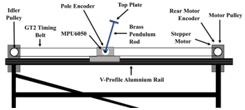
Figure 1. Schematic diagram showing main pendulum components.

2. Mechanical design of the Inverted Pendulum

2.1.  Extension of previous work

The current inverted pendulum design expands upon our previous publication [1], in several important ways. We made modifications to the mechanical components of the pendulum system, enabling us to alter its physical characteristics and now utilize a range of pendulum configurations, with changes in pendulum length (635mm, 335mm, 233mm), viscous damping (adding a paddle to the pole), and friction (compression of a brake on the pendulum pole).

2.2.  Inverted pendulum components

Here we build an inverted pendulum system consisting of a pole pivoted at one end on a cart that moves on a linear track actuated by a stepper motor, which can be balanced in its inverted position by observing the pole angle and controlling cart movement. Our design comprises several distinct component parts, illustrated in Figure 1.

The pendulum assembly is composed of several distinct components. These include a v-groove aluminum profile track and a cart unit that supports the inverted pendulum, moving along the track on a wheeled cart. Additionally, a stepper motor unit propels the cart via a timing belt from one end of the track, while a passive idler pulley supports the belt at the opposite end. The motor and pulley mechanisms are securely affixed to the aluminum profile structure using T-nuts. This design not only offers the flexibility to easily remove and replace these parts with similar components but also simplifies the process of tensioning the drive belt.

2.3.  Track

The mechanical design integrated a V-slot profile to realize the pendulum track. This streamlined construction since it enabled the use of readily available accessories. These included a stepper motor mounting plate, an idler pulley mechanism, as well as gantry plates.

2.4.  Cart

A 4-wheeled gantry plate formed the basis of the cart mechanism. During balancing operation, it traversed the V-slot aluminum track along its sides as needed to balance the pendulum pole. Wheel clearances were adjusted so the cart remained securely on the track without excessive wobbling, while also avoiding undue friction.

A thick flat PLA+ 3D-printed rectangular sheet with mounting holes was affixed to the gantry plate. This served as the support for both a ball bearing race and an encoder unit, which held and facilitated the rotation of a shaft. This shaft, in turn, held the pendulum pole, allowing it to swing freely. The incremental encoder measured the pole’s angular deviation from the vertical position, as depicted in Figure 2.

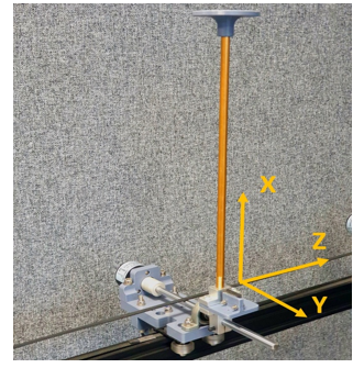
Figure 2: 3D-printed pendulum cart incorporating an encoder and an inertial measurement unit (IMU). A flat-topped table can be attached to the end of the pendulum to support objects on its surface.

2.5.  Shaft friction adjustment

Normally, the rotation of the pendulum shaft is resisted by a low level of friction, arising from the bearing and the incremental encoder. To increase the amount of friction and examine its effect on pendulum behavior, a spring-loaded braking assembly was constructed (Figure 3). This consisted of a semicircular brake pad section made of PLA+ that could be pressed against the pendulum rotary shaft using a compression spring, thereby hindering its rotation. By fully withdrawing the brake, it was also possible to remove its effect completely.

2.6.  Standard pendulum pole

The standard pendulum pole consists of a pole crafted from a brass segment, selected for its easy machinability and high density. One end of the pole was threaded to securely screw into an attachment component connected to the main shaft, ensuring a sturdy attachment as depicted in Figure 2. This led to an overall pendulum length of 335mm. While a relatively short pole increases the balancing challenge, necessitating quicker cart reactions due to the system’s elevated natural frequency, it yields several benefits. A compact pole is not only more manageable but also ensures increased safety by minimizing accidental impact risks. Moreover, it provides characteristics that better match other systems, like smaller balancing robots [60].

2.7.  Additional pendulum poles

An easy way to alter the fundamental characteristics of the pendulum is to change the length of the pole. To do so, two additional pendulum poles were built (Figure 4). These poles consisted of 8mm diameter stainless steel poles, leading to pendulum lengths of 222mm and 635mm. Since they were only required for intermittent use, no screw attachment was used, thereby facilitating construction. Instead, they were simply clamped at their endpoint into another attachment component connected to the main shaft.

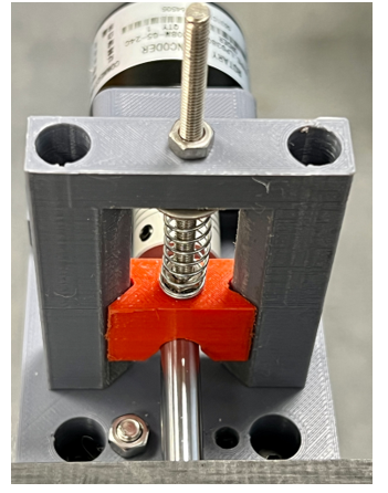
Figure 3: Shaft friction adjustment mechanism for the pendulum cart, designed to alter the sliding friction around the pendulum’s rotational axis.

2.8.  Pendulum pole end attachments

To provide a platform for placing objects, and to shield its endpoint for safety reasons, a round disc was 3D printed from PLA+ and slid onto the end of the pendulum pole, where it was held in place by friction.

To offer a means to change the viscous air resistance experienced by the pendulum pole as it swung, the round disc at the endpoint of the pole could be replaced with a paddle (Figure 5). The paddle consisted of a 5mm thick square measuring 100mm by 100mm and was 3D printed from PLA+. It slid onto the end of the pole via a central mounting hole and was again held in place by friction. By rotating the paddle 90°, it was possible to adjust the amount of viscous resistance the pendulum pole experienced from a low to a high value.

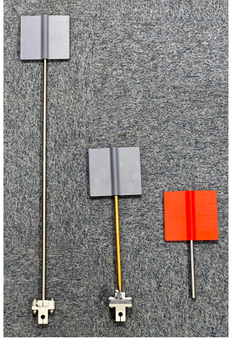
Figure 4: Three different pendulum poles were utilized to evaluate the controller’s sensitivity to changes in pendulum length.

2.9.  Stepper motor actuation

The motor drive assembly includes an aluminum plate, situated on the profile rail, which serves as firm support for a NEMA23 stepper motor. The motor is securely affixed to the plate using bolts. The motor is connected to a drive pulley at its front, and an encoder is mounted on the rear end of its shaft. This enables accurate measurement of the cart’s position, although it is only needed to analyze the pendulum’s behavior and is not involved in the balancing process (see Figure 6).

To operate the stepper motor, an A4988 stepper controller is employed, driven from an Arduino Mega 2560 R3 Microcontroller. The latter is programmed in C++ and provides precise control of the pendulum cart along the linear rail.

2.10.           Belt

A pulley and belt mechanism are used to convert the motor’s rotary motion into linear movement, thereby appropriately driving the cart along its rail. The cart traverses its designated rails using a GT2 timing belt, which is typically used in 3D printers. The belt, affixed to the cart using steel clamps, spans almost the entire length of the track. The stepper motor, located at one end of the track, has a 60-tooth GT2 motor pulley secured to its shaft. A passive idler pulley is situated at the opposite end of the track. Ball bearings, integrated into the idler pulley, minimize frictional resistance, ensuring smooth operation even under the stress of high belt tension. Adjusting the precise location of the idler provides an easy means to modify belt tension.

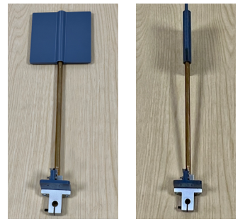
Figure 5: The pendulum paddle can be rotated, thus adjusting the viscous drag due to air resistance from low to high values.

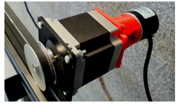
Figure 6: Stepper motor actuation, showing the drive pulley and a custom-made 3D-printed encoder mount at the motor’s rear.

2.11.           Inertial Measurement Unit

To support future developments of the pendulum system, a cost-effective 6-DOF accelerometer/gyro (MPU-6050) was strategically mounted to a 3D-printed support on the pendulum pole, aligning it with the pendulum shaft’s rotational axis. This configuration presents an alternative method to measure the pole’s angular displacement. The pendulum shaft’s rotation revolves around the MPU-6050’s y-axis. When in the inverted configuration, its x-axis points downward, and the pole points upwards along its negative x-axis, with its z-axis horizontal (Figure 2).

2.12.           Modular adjustable pendulum design

The utilization of modular construction within the system ensures that the parameters governing the behavior of the inverted pendulum can easily be adjusted or reconfigured. Such adaptability can prove useful in educational contexts. With minimal adjustments to the apparatus, diverse tasks can be allocated to distinct student cohorts, each tackling a specific control problem. For instance, the pole’s length, an essential aspect of the system’s dynamics, can be altered by substituting the pole with another of a different length. Adaptability extends further to the motor unit. For example, stepper motor drive could be exchanged with actuation employing a BLDC motor, a modification that would support force control, as opposed to velocity control, of the pendulum system.

2.13.           3D printing

The components for the pendulum cart were designed using AutoCAD Fusion 360. This software also facilitated the conversion of the designs into STL format files, which is a critical step for additive manufacturing. The mechanical parts were then fabricated using PLA+ material on a Creality 6SE 3D printer. It is noteworthy to mention that although tougher plastics could further enhance the durability of the design, PLA+ was chosen for its ease of printing and cost-effectiveness.

2.14.           Pendulum Stand

Operating the pendulum necessitates mounting the track at an elevation that ensures unobstructed swinging of the pole. We designed a custom-engineered support stand using aluminum profiles to secure the pendulum system (refer to Figure 7). This stand offers a robust yet lightweight construction that facilitates easy transportation.

The support stand comprises two support pillars, fabricated from aluminum profile. These pillars are anchored at their base with additional lengths of aluminum profile, and 3D printed feet are used at each end to provide stable support. The top of each pillar is fitted with a 3D-printed bracket, tailor-made to accommodate the aluminum v-rail. To enhance the rigidity of the structure and to increase its resistance to mechanical stress, diagonal aluminum profile sections are incorporated, to brace the assembly. This results in a rigid structure, minimizing potential vibrations or displacements that could affect the system’s performance.

3. Mechanical tapper for performance evaluation

3.1.  Testing balancing systems

Monteleone and his team [61] presented a methodology to evaluate the balance resilience of robots, utilizing unique performance indicators and a custom-made testbed. Through extensive testing on a humanoid robot, their study demonstrated the method’s effectiveness in designing more robust robotic systems.

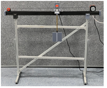
Figure 7. Pendulum mounted on its stand: The structure uses diagonal bracing to increase its rigidity.

3.2.  Tapper components

In the same vein, to conduct tests across various pendulum conditions, including different pendulum lengths, friction, and damping levels, as well as different control laws, and to compare the results, it was necessary to disturb the pendulum pole consistently. To achieve this, a tapping mechanism was constructed (Figure 8).

We built and used a testing rig to deliver repeatable disturbances to the pendulum pole whilst balancing, to examine the recovery and robustness of control. This could be carried out during balancing whilst the cart was either static or moving.

3.3.  Finger-spring mechanism

The primary component of this tapping mechanism is the ‘tapper finger,’ which is mounted onto a baseplate. This mounting baseplate for the tapping mechanism is attached to a cart that can be maneuvered up and down a V-groove rail track by means of a stepper motor.

The finger is composed of a stainless-steel pole inserted in a PLA+ holder, which pivots around a rotary axis located 3 cm from its lower end. Two sets of springs are connected at the endpoint of the holder and at the base on either side, pulling in opposite directions. When the finger is in its undisturbed equilibrium position, these springs ensure that it maintains a 0° orientation.

This finger-spring assembly forms an underdamped second-order system. Its behavior, particularly the overshoot following appropriate excitation, serves as an effective method to strike the pendulum pole. To generate a movement suitable for producing a tap, it is necessary to displace the lower end of the finger from its equilibrium position around its pivot and then release it suddenly. This action results in a rapid movement: the finger travels back through its equilibrium position and out the other side, which enables it to impact the pendulum pole and then quickly withdraw.

Using this tapping mechanism, it is important to note that the pendulum pole must be positioned at an appropriate distance from the tapping finger before operation commences, to prevent multiple impacts. At the tap, energy is transferred from the finger to the pendulum pole, and if the distance to the target pendulum pole is set correctly, it ensures that the finger only strikes once and then retreats without making further contact.

3.4.  Finger actuation

Although it would be possible to manually displace the lower end of the tapping pole and release it by hand, we incorporated an RC servomechanism into the design to achieve this action automatically and more consistently. The RC servo first displaces the finger from its equilibrium position. Then, owing to the cam mechanism’s design, it releases the finger suddenly as it passes the end point. This action consequently results in a rapid underdamped second-order trajectory of the end of the tapper finger, ideal for exciting the pendulum pole.

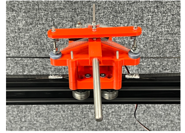
Figure 8. 3D-printed tapping mechanism. Two sets of springs are configured to pull the bottom of the tapping pole to the left and right, thereby establishing a neutral equilibrium position at 0° as depicted. An RC servo is positioned to travel 180°, engaging and then releasing the rear of the tapping mechanism. This action, assisted by the tension of simultaneously contracted springs, causes the pole to swing in an under-damped motion, with overshoot delivering an appropriate tap to the pendulum pole. All custom parts were designed using AutoCAD Fusion 360 and printed with PLA+ material.

To achieve a consistent tap, it is essential to maintain a constant distance between the tapping pole and the pendulum pole and to ensure that the tap occurs at the same location during each trial. This consistency is achieved by visually aligning the tapping finger with the pendulum pole before a tap is initiated.

3.5.  Tapper cart

In the inverted pendulum position control mode, the pendulum cart remains stationary, simplifying the process of tapping its pole. However, in the velocity control mode, the cart moves along the rail while balancing. The goal was to create a tapping mechanism suitable for both velocity and position modes, necessitating the ability of the tapping mechanism to track the pendulum cart’s movement by employing an additional cart. This capability ensures taps can be delivered effectively, even while the pendulum cart is in motion. To achieve necessary synchronization, the tapping mechanism’s cart is propelled along a separate V-groove aluminum profile track, using a stepper motor that receives the same control signal as the pendulum cart’s stepper motor.

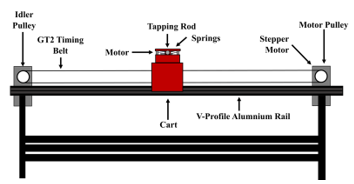
Figure 9. Schematic of the tapping mechanism mounted on its adjustable stand, showing all its main components.

3.6.  Adjustable height tapper stand

The upper track of the tapper mechanism was mounted to the side of the support pillars, allowing for adjustable height of the tapper, as illustrated in Figures 9 and 10.

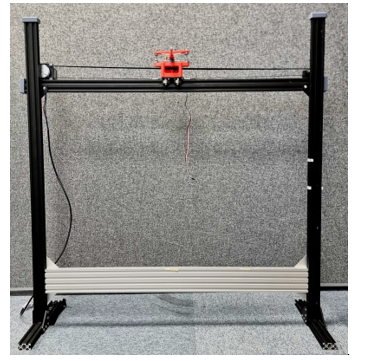
Figure 10. Side view of the adjustable mechanical tapper assembly. The cart supporting the tapping mechanism can be driven left and right to synchronize with the pendulum cart. The cart is mounted on a rail that can be slid up and down the outer stand legs, and then fastened firmly in place with screws, enabling adjustment of the height at which tapping occurs.

4. Analysis of pendulum dynamics

4.1.  Mathematical analysis

We performed a comprehensive analysis of the pendulum’s dynamics, including the nonlinear differential equation, its linearization, and s-domain representation. This provided a theoretical foundation for our practical implementation.

4.2.  Equilibrium positions

A pendulum exhibits two distinct equilibrium points. In the stable equilibrium state, the pendulum hangs downward, functioning like a traditional pendulum, similar to those in pendulum clocks. At this stable equilibrium point, if the pendulum is slightly displaced, it will begin to oscillate back and forth with a characteristic frequency determined by its dynamic properties. Factors such as damping in the joints and air resistance lead to a gradual decrease in oscillation amplitude over time. Eventually, the pendulum will stop moving and return to a stationary state at its equilibrium position. In contrast, an unstable equilibrium occurs when the pendulum is delicately balanced upright on its pivot point.

4.3.  Analysis of non-linear pendulum dynamics

If sliding friction is neglected, the kinematics of an inverted pendulum can be characterized by the following non-linear differential equation:

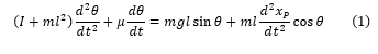
Here, the terms represent the following:

θ: Angle of the pendulum pole to the vertical axis

μ: Coefficient of viscosity

m: Mass of the pendulum

I: The Moment of Inertia (MoI) of the pendulum pole about its center of mass

l: Distance from the pivot point to the pendulum pole’s center of mass (typically half the length of the pole)

x_p​: Displacement of the pivot

Although exponential decay due to viscous resistance is often assumed to be the primary cause of oscillatory decay in second-order systems like the pendulum, it is known that sliding friction leads to a linear decay of oscillatory amplitude [62–65]. To account for sliding friction, we can also write

In this context, an additional friction term exists, scaled by the coefficient f, which is dependent on the sign of the angular velocity. The presence of this sign term complicates formal analysis; therefore, we initially disregard the effects of friction.

We observe that the provided kinematic description suffices for deriving control, assuming reliance solely on the cart’s velocity as the control input. Additionally, it’s worth noting that force control, a common approach in numerous inverted pendulum implementations [66], would necessitate an extra equation to accurately capture the dynamics of the cart’s force.

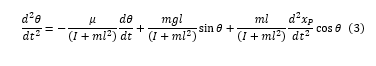
Refactoring Eqn. (1) with the highest-order differential term on the left-hand side, yields:

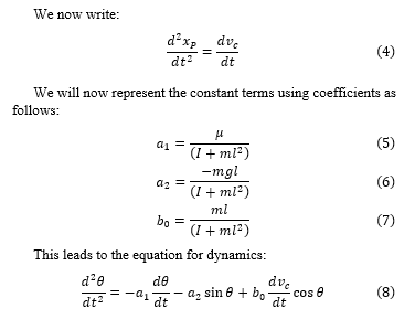
To express the system in state space form as two first-order differential equations, selecting the first state x₁​ ​is straightforward since it represents the pendulum angle, denoted as θ:

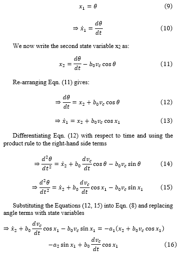
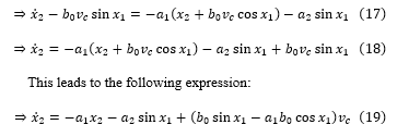
The two equations (13) and (19) can be used in a non-linear simulation of the pendulum system.

5. Linearizing the non-linear system

5.1.  Equilibrium

We now extend the mathematical analysis to derive the linearized state space model by calculating and evaluating the system’s Jacobian around equilibrium positions. To linearize the nonlinear differential equation description of the pendulum around its equilibrium points, we first need to identify their locations. Equilibrium occurs when the control input is zero, and the state derivatives are also zero. That is

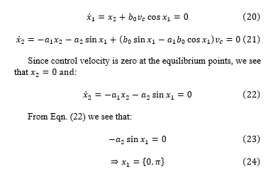
Thus, the system has an equilibrium in an inverted configuration at 0 radians and a non-inverted configuration at π radians. To linearize the system at these equilibrium points, we need to calculate the Jacobian of the system, denoted as , with respect to the system state, and evaluate it at those points. We first express the two state equations as functions:

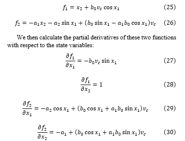
5.2.  Jacobian in matrix form

This leads to the Jacobian matrix:

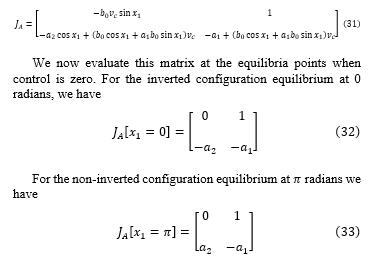
We now need to linearize the control of the system. To do so, we calculate the Jacobian of the control, denoted as , with respect to the control input. This involves calculating the partial derivatives of the two system functions with respect to the control input.

5.3.  Linearized ODE

Multiplying out the matrix Equations (41, 42), we see that we have two linear equations. For the first state, we have:

5.4.  System eigenvalues and stability

The eigenvalues (λ) of the system matrix A represent the behavior of the pendulum system. These eigenvalues are related to the poles in the transfer function. The eigenvalues, denoted as λ, of matrix  can be determined by solving the following matrix equation, involving the calculation of the determinant, where  is the identity matrix:

If all eigenvalues have a negative real part, the system will be stable. Conversely, if any eigenvalue has a positive real part, the system will be unstable. It is also important to note that if the real part of an eigenvalue is zero, then the system is marginally stable, existing on the boundary of stability, neither conclusively stable nor unstable. Complex eigenvalues typically lead to oscillatory behavior, especially if they have a non-zero real part.

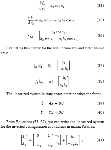
To incorporate feedback control into this system, the system must use a feedback mechanism. One approach involves utilizing full state feedback, as depicted in Figure 11. In this figure, the matrix K represents the gain of the state feedback, while R(t) denotes a reference input. If the reference input is zero, the state feedback can be described by the following expression:

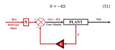
Figure 11. Signal flow graph of a plant under direct full-state feedback control: The red line delineates the feedback path, which includes multiplication by the feedback gain, denoted by K. Additionally, a feedforward gain term, represented by , is introduced to improve tracking of the reference input.

Substituting the state space system equations (39) and (40) into this expression leads to the modified state space equations, which represent the system dynamics under the influence of the feedback mechanism.

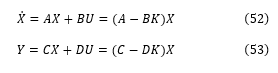
Implementing state feedback alters the system dynamics leading to a new expression for the state derivative. This alteration involves not just multiplying the state by matrix A, but rather by (A−BK). Consequently, the eigenvalues (λ) of the full state feedback system can be determined by solving the updated characteristic equation:

Consequently, by modifying the gain matrix K, we can manipulate the location of the system’s eigenvalues. The method for calculating K is discussed in Section 7.

5.5.  Using a Luenberger observer

Many procedures in control design assume that the full state vector is available. However, this is often not the case, as in our pendulum design. In such circumstances, we can use an observer to estimate the full state using a linear plant model. The Luenberger observer computes the state estimate according to the differential equation:

The observer uses the state space matrices A and B to provide a linear model of the plant. In our case, we determine the observer gains, denoted as L, using MATLAB. Similar to the state feedback gain, the Luenberger observer gain vector L must be chosen such that all the eigenvalues of the observer system, as solutions to the characteristic equation, possess appropriate negative real values. The signal flow graph for the Luenberger observer is shown in Figure 12. The system’s eigenvalues satisfy the following characteristic equation:

The calculation of L is discussed in Section 7.

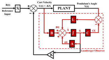
Figure 12. Estimation of plant state using a Luenberger observer. The observer, which simulates the real dynamics of the inverted pendulum, generates an estimated state, denoted as . This estimated state serves as a proxy for the actual system state, labeled X, some of which may be unobservable. The signal Y(t) is employed to correct the state estimate.

6. Augmenting the state space model

6.1.  Adding cart positional state

To enable control of both the cart’s position and the balancing of the pole, we introduce an additional state variable x₃ to explicitly represent the cart’s position. We can relate the cart position to the control velocity input, since:

We can compute the numeric values of the matrices using MATLAB. See Figure 13 for the udpated state feedback controller signal flow graph schematic.

6.2.  Adding integral action

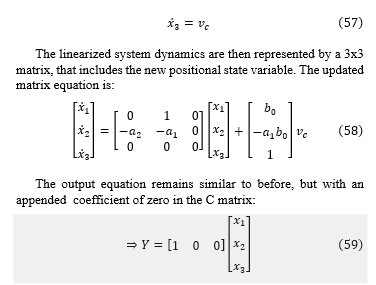
We can further improve cart position performance and reduce its steady-state error by adding integral action on the cart position (see Figure 14). To incorporate integral action, a state is devised within the controller to compute the integral of the positional error signal. This is then used as a feedback term, as denoted by the red path on the schematic. Therefore, to achieve integral feedback, we simply augment a state-space system by adding another state Z, whereby the state Z is the integral of the error between the desired output ref_p (representing a reference input for cart position) and actual output Y. Thus, the standard state-space equation:

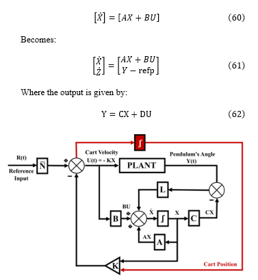
Figure 13. Adding a state for cart position provides a means to control cart position.

State feedback control is now generated from the state X and also from the state Z. That is:

Thus, to add integral action to the state-space model of the cart position-augmented pendulum, and use the cart position to generate error integrated over time, we further augment the system matrices given in Eq. (58). We add a fourth state, x₄​, to represent the integrated cart position error.

Notice that here we update the integral state by selecting the position state x_3​ to generate the (Y− ref_p) term used for integral action. For this model, we assume the reference position, ref_p, is zero.

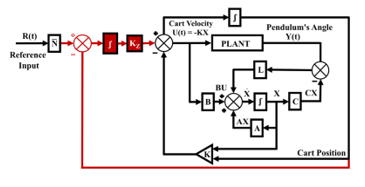
Figure 14. Illustration of integral error feedback within the system. This mechanism reduces steady-state positional error of the cart by comparing the reference setpoint with the estimated cart position, integrating the positional error, and using it in the feedback path.

7. Designing state feedback controllers

7.1.  Determining feedback gain

In our pendulum design, a linear full state feedback controller is employed to balance the inverted pendulum. This method enables the maintenance of balance, even in the presence of noise and disturbances. Implementing this controller requires obtaining K, the feedback gain vector.

Various strategies can be used to find K. One method is to use pole placement, whereby we calculate K in order to achieve what we consider to be a good choice of poles for the system when it is operating under full state feedback control. Alternatively, the gain K can be found by formulating gain calculation as an optimization problem, where we specify an objective function indicative of what we consider desirable performance should be. In this work, we adopted the latter optimal control approach. Specifically, we find the gain K utilizing the MATLAB lqr command (which designs a linear quadratic regulator).

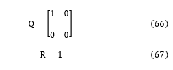
7.2.  Velocity control mode

To design an optimal controller to balance the inverted pendulum using velocity as the control input, we need to consider the linear 2 state model given by the equations (41) and (42). To build an appropriate cost function for the optimization, suitable values were implemented along the leading diagonal of the 2×2 Q matrix to penalize non-zero system states. In addition, a suitable value is used in the 1×1 R matrix to penalize the control input.

Penalization of the state serves a crucial function: It ensures that the system approaches its target value. Within the scope of this design, it assists in keeping the pendulum’s angle close to zero, facilitating effective balancing. In contrast, penalizing control with R serves to reduce the speed of the cart. The penalization values were determined  through experimentation.

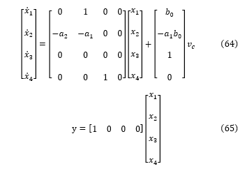
7.3.  Position control mode

To implement the control of the cart position as well as balancing the pendulum pole, we make use of the 4-state system that incorporates integral action. The linear state space system is described by equations (64) and (65). The diagonal entries of the 4×4 Q matrix, along with the single scalar value in the R matrix, were defined to aptly penalize state and control. The penalization values in Q and R were found by trial and error.

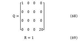
To concurrently accomplish pendulum balancing as well as control of the cart position, we applied a larger penalty on state x₄​ (which represents the integral of positional error), whereas state x₃​ (which represents cart position) received a penalty term of zero.

7.4.  Designing the Luenberger observer

To determine the Luenberger gain L, we again employed the MATLAB lqr command. We refrained from using the observer to predict the cart’s velocity or position since estimating these is straightforward, given that velocity is directly used as the control signal.

As with the determination of state feedback controller gains, the leading diagonal entries of the 2×2 Q matrix and the single value in the R matrix were selected to penalize the system states and the control action, respectively. Suitable parameter values for these matrices were ascertained through trial and error.

7.5.  Gain scheduling

Transitioning between velocity control of the pendulum and position control of the pendulum was realized by selecting their respective system gain K and pre-processing term  (as discussed later and presented in Table 2). We note that resetting the integral error state to zero was necessary each time the controller was switched from velocity to position mode, to ensure processing started with a zero positional error.

In position control mode, we make use of integral action. In this case, the reference position input can have a zero value to preserve the cart’s current position on the track.

During the velocity control of the cart, the velocity of the cart is required to track the reference input. To ensure this takes place the controller requires an appropriate feedforward pre-emphasis term, denoted as :

For velocity control, we note that   has a value of 1 (that is, a gain of unity). Thus, the reference input directly sets the cart velocity. This is achieved by a slight update to the calculation of the control signal, which now incorporates a non-zero reference input, referred to as ‘ref’:

8. Laplace Analysis of the Inverted Pendulum Dynamics

8.1.  System transfer function

Laplace analysis can provide useful insights into system behaviour. Neglecting the non-linear effect of friction, the linearized  differential equation that describes the  pendulum can be expressed as:

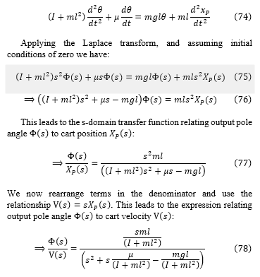
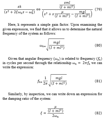
8.2.  2^nd order canonical form

Comparing the expression with the second-order canonical form, we can identify the coefficients and characteristics of the system. This comparison allows us to further analyze the dynamics of the inverted pendulum and gain deeper insights into its behavior and control requirements.

 

9. Numeric integration to implement real-time control

9.1.  Euler integration

To implement real-time state feedback control, some form of numerical integration is needed. Such integration can often be carried out satisfactorily on a digital computer using Euler’s methods. Forward Euler integration works by incrementally calculating contributions to the integral that arise from the differential term.

The basic idea is as follows. Consider a function y=f(x) such that when x=x₀ then y=y₀. This is illustrated in Figure 15. As we increase the value of x by Δx we reach a point where x₁=x₀+Δx and similarly this increases y by Δy reaching the value y₁=y₀+Δy. Therefore:

The gradient of the curve at (x₀, y₀) is the tangent at this point. From Figure 15, it is seen that the gradient at this point can be approximated by the ratio of a small change in y divided by a small change in x:

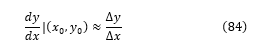
This is only strictly true in the limit where Δx tends to zero. In practical numerical methods, this limit is approximated by choosing a sufficiently small Δx. We also see that we can use this relationship to iteratively estimate y₁ from y₀ by replacing the Δy term by two very close and successive y values:

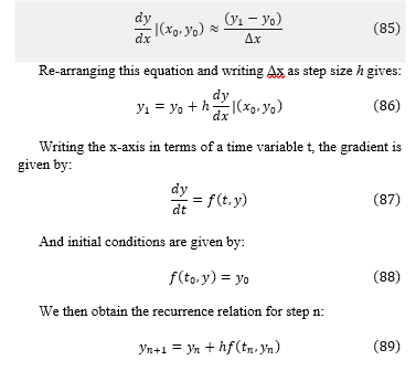
Where t is time, at initial time to the output is y₀, at future time t_(n+1) the output is y_(n+1), and h is the step size. This expression can be used to iteratively find the next estimate of y₁ if we know x_o and the gradient at (x₀, y₀). This approach provides a method for integrating the differential term, which is generally satisfactory if a sufficiently small temporal step size, h, is used. This method is easily extended to vector form to perform the integration stage needed in state space models.

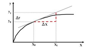
Figure 15. The gradient dy/dx​ of a curve y=f(x) can be locally approximated at the point (x₀​,y₀​) as the ratio of a small change in the value of y to a corresponding small change in the value of x.

9.2.  Higher order numerical integration

Euler integration is the simplest fixed-step numerical method that can be adopted. However, other more complex integration rules can also be used. These include the midpoint, trapezoidal, and Runge-Kutta methods, which, though requiring more computational steps in the estimation of the integral, offer higher accuracy. Additional methods utilize dynamic selection of step size, such as the ode45 function in MATLAB. See [67] for a discussion of these methods.

Here, we use MATLAB’s ode45 for simulations of the uncontrolled stable pendulum configuration. We use Euler Integration to model the controlled pendulum because of the method’s simplicity and its ease of implementation on a microcontroller, especially considering its low computational requirements.

10. System identification

10.1.           Large angle pendulum oscillatory behavior

Approximately estimating observable parameters of a pendulum, such as length and weight, can be done with relative ease. However, assessing other parameters is considerably more challenging, and in some cases, impossible, solely based on observations of the static mechanical system. To accurately determine values for viscous and sliding friction, it is necessary to conduct measurements during pendulum movement.

To examine the large-angle oscillatory behavior of the pendulum, we raised it from its resting, vertically hanging (non-inverted) position to a horizontal alignment, corresponding to an angle of approximately 90°, before releasing it. The pendulum then oscillated until viscous damping and friction gradually brought it to a standstill in its vertical, non-inverted position.

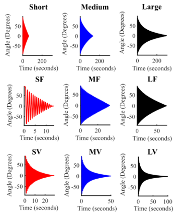
Figure 16. Pendulum large angle oscillation decay over time for three pendulum lengths. Data captured using an incremental encoder.  Top row: No added viscosity or friction for short, medium, and long pole lengths. Middle row: Effect of added friction for short, medium, and long pole lengths (SF, MF, and LF, respectively).  Lower row: Effect of added viscosity for short, medium, and long pole lengths (SV, MV, and LV, respectively).

10.2.           Data logging

To examine the pendulum’s oscillation decay over time, we collected time-stamped pole angle data from its shaft encoder as the pendulum swung. In addition, the pendulum cart position was recorded using readings from the encoder mounted on the rear of the cart drive stepper motor. The data were gathered using a program running on an Arduino Mega, which transmitted the time and angular measurements to a host PC equipped with Microsoft Excel. The Excel program was used to record the data at a 25Hz rate and save it to the hard disk in Excel file format. Subsequently, the data were imported into MATLAB for analysis. This allowed for the generation of a plot depicting the pendulum’s decaying oscillations under various conditions, as well as further analyses.

The mechanical pendulum system features three interchangeable poles, and for each pole, the level of friction could be adjusted from low to high. Similarly, the viscous damping could be altered from low to high by manipulating the wind resistance experienced by the paddle mechanism. This configuration led to a total of 9 different experimental conditions.

Figure 16 top row shows the temporal response waveforms for the undamped cases with no added friction for all three pendulum lengths, plotted on the same scale. It is observed that a longer pendulum length significantly increases the time required for the pendulum angle to decay to zero. Figure 16 middle and lower rows illustrate the responses of pendulums of three different lengths with additional friction and additional viscosity introduced, respectively. It is apparent that incorporating viscosity into the system accentuates the exponential decay. However, it is noteworthy that when friction is the dominant factor, the decay is linear rather than exponential.

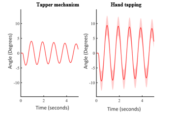
Figure 17. Testing the consistency of the tapping mechanism. Mean and standard deviation of the pendulum angular response averaged over 8 trials are shown using the tapper mechanism and hand excitations of the pendulum pole.

10.3.           Small angle pendulum oscillatory behavior

The primary interest of this study is the examination of the balancing behavior of the pendulum system in its inverted configuration; therefore, large angle behavior is not of particular relevance. In a balancing configuration, the pendulum pole is maintained close to its unstable equilibrium position by the controller. In this case, the angular deviation from the 0° position is small, which is also essential for the validity of the linear approximation made in the observer model. Therefore, to estimate the parameters of the linear model accurately, it is necessary to examine the pendulum operation at small angles of deflection and to perform system identification for all pendulum parameters under these conditions. To generate consistent excitation to the pendulum, we utilized a mechanical RC servo tapping mechanism.

11. Using the tapping mechanism

11.1.           Evaluating tapper consistency

To evaluate the consistency of the tapping mechanism’s operation, we conducted tests on the medium pendulum pole without added friction or viscosity. Figure 17 illustrates that the tapper provides very consistent excitation of the pendulum, particularly when compared to the variability typically observed with manual tapping by hand.

11.2.           Excitation of non-inverted pendulums

We examined the pendulums in their normal, stable, hanging-down mode to characterize the effects of the tapping. Figure 18 illustrate the responses of pendulums of different lengths driven by the tapper mechanism, both with and without added friction and viscosity. In comparison to the large angle oscillation tests, it is noteworthy that at small angles, the paddle has only a minor effect, and additional friction more rapidly damps out pendulum oscillation.

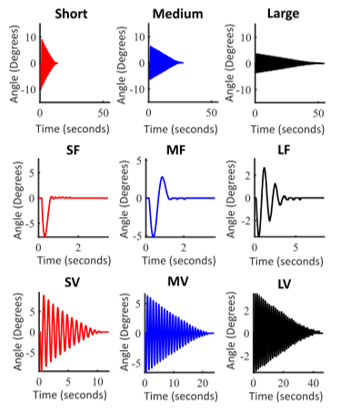
Figure 18: Pendulum small angle oscillation decay over time. Top row: No added viscosity or friction. Middle row: Effect of added friction for short, medium, and long pole lengths (SF, MF, and LF, respectively). Lower row: Effect of added viscosity for short, medium, and long pole lengths (SV, MV, and LV, respectively).

11.3.           Estimating pendulum parameters

We performed grey-box system identification of the physical pendulum mechanism to identify parameters of viscous and static friction, and to fine-tune others, including pendulum length, weight, and moment of inertia.

To fit the small angle pendulum response data, we focused on six of the nine configurations: the three pole lengths both with and without added viscosity. This fitting was accomplished with a simulation of its nonlinear dynamics, employing an optimization procedure using the MATLAB fmincon function. We discarded the configurations with extra friction due to the dramatic impact it had on the system’s behavior, which resulted in a limited amount of useful temporal data. This procedure optimized the mass, effective pole length, pole moment of inertia, sliding friction, and viscous friction parameters of the pendulum system.

We designed an objective function that minimized the sum of squared distances between the predicted oscillations and the measured data. To align the simulation with the measured data for comparison, we first trimmed the measured data to begin at its first positive peak in the pendulum’s oscillation. The pendulum’s angular velocity at this point is zero, and its corresponding angle was used to set the initial angular state in the non-linear simulation of the pendulum, based on Eqn. (2), that includes both viscosity and friction. This was carried out using the MATLAB ode45 solve.

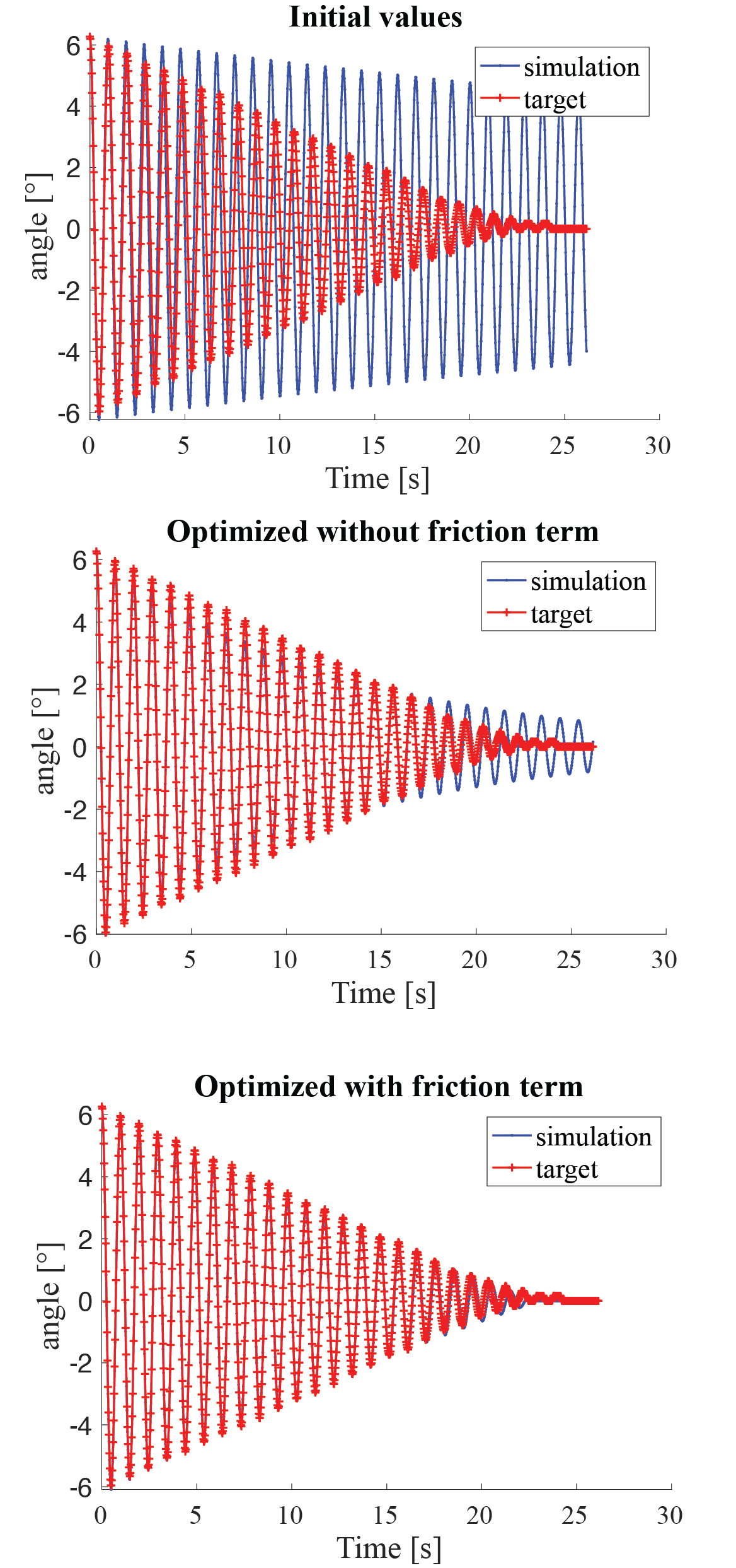
Figure 19. Running optimization to fit the measured response of the medium-length non-inverted pendulum without additional viscosity or friction. Top plot shows the predicted response based on an initial rough guess. Middle plot shows the estimated response after running the optimization algorithm without including the friction term. Lower plot shows the estimated response when the friction term is present. It is evident that accounting for friction leads to a significantly better fit.

We initialized the simulation parameters based on direct measurements of pendulum pole length and mass. Initially, we estimated the values of the friction and viscosity parameters through a process of trial and error, which was aided by careful observation of the simulated responses. During the fitting procedure, we allowed the optimization algorithm to refine all parameter values. However, it was necessary to constrain the parameter solutions to prevent fits that deviated substantially from the known ground truth values for mass and pendulum length. To this end, the mass and length were constrained to values between 0.9 and 1.1 times their measured values. The other parameters, for which we had less grounded certainty, were allowed to vary from 0.1 to 10 times their initial estimated values.

Table 1. Physical Measurements of the three different pendulums and estimated values found by system identification. Values marked with ‘F’ represent estimates with friction included in the second-order nonlinear differential equation model of the pendulum. The bold values represent estimates made when only a viscous damping term is present.

	Short Pendulum		Medium Pendulum		Long Pendulum
	Normal	Viscous	Normal	Viscous	Normal	Viscous
Measured Length to CoG [m]	0.233/2 = 0.117		0.335/2 = 0.168		0.635/2 = 0.318
Measured Weight [Kg]	0.174		0.226		0.336
Estimated Half-length to CoG [m]	0.116(F) 0.106	0.117(F) 0.105	0.167(F) 0.149	0.164(F) 0.149	0.322(F) 0.317	0.308(F) 0.316
Estimated Weight [Kg]	0.178(F) 0.158	0.174(F) 0.157	0.207(F) 0.207	0.202(F) 0.207	0.341(F) 0.338	0.327(F)x 0.338
Estimated MoI [Kg-m2]	8.97e-04(F) 9.02e-04	8.47e-04(F) 8.83e–04	0.0024v 0.0027	0.0024(F) 0.0027	0.0142(F) 0.0144	0.0147(F) 0.0146
Estimated Viscosity [N-m-s/rad]	2.21e-04(F) 9.90e-04	2.22e-04(F) 1.00e-03	3.36e-04(F) 1.00e-04	2.35e-04(F) 1.00e-04	2.22e-04(F) 0.0038	5.20e-04(F) 0.0048
Estimated Friction [N/Rads-1]	5.05e-04(F) n/a	6.16e-04(F) n/a	3.07e-04(F) n/a	3.87e-04(F) n/a	3.87e-04(F) n/a	5.46e-04(F) n/a

Figure 19 shows the results of using system identification to fit model parameters to the measured data for the medium-length, low-friction, low-viscosity pendulum condition. The initial guess, which incorporated insufficient damping, is shown in Figure 19 top plot. A reasonably good fit is achieved by fitting the model with only viscous damping, as demonstrated in Figure 19 middle plot. An even better fit is obtained when the model also includes sliding friction, depicted in Figure 19 1ower plot.

For each pendulum length, measured and estimated values were obtained, both with and without friction, leading to a total of six conditions. These conditions are presented in Table 1. The corresponding (no-friction) state space matrices and Luenberger gain L are shown in Table 2. The computed state feedback controller system gains K and reference pre-scaling factor , are shown in Table 3.

11.4.           Reality check using canonical form

To provide a ballpark estimate of the main parameters of the three pendulums in their low-damping modes, each pendulum was first nudged using the tapper mechanism and then allowed to sway freely, eventually settling into its stable position, as depicted in Figure 20. Measured values are shown in Table 4.

Table 2. Values of the state-space matrix and Luenberger observer gain, presented in MATLAB syntax.

Parameter	Value
A
B
C
L

Table 3. Computed state feedback control K gains and  values used for the two control mode (in MATLAB syntax).

Control 1zModes	K Gain
Position Control		0
Velocity Control		1

Table 4. Measured decay and nearest integer number of cycles as a function of time for all three pendulum lengths in undamped conditions. The values in brackets were found by the system identification procedure.

	Short Pendulum	Medium Pendulum	Long Pendulum
Measured Maximum Time [s]	13.50	27.0	54.8
Measured 50% Decay Time [s]	5.99	12.15	26.2
Measured 50% Decay Cycles [integer count]	7	12	19
Observable frequency of oscillation fd [Hz]	1.17 Hz (1.25 Hz)	0.99 Hz (1.03)	0.73 Hz (0.74 Hz)
Estimated damping ratio ζ	0.016 (0.024)	0.0091 (0.011)	0.0057 (0.0084)

We used Equations (80 and 81) to calculate the corresponding natural frequencies, which were essentially the same as the damped frequencies due to the very small damping ratio. These values aligned well (within 10%) with those obtained through system identification, confirming the appropriateness of the values found by the fitting procedure. We calculated the damping ratio from the decay to 50% in a time using the equation:

From Table 4 it can be seen that the system identification yielded similar values.

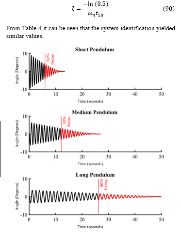
Figure 20. Approximate estimation of the canonical parameters for the pendulum system by observing the frequency of oscillation and the amplitude decay to 50% of the initial value. Plots are shown here for the short, medium, and long-length pendulums (with no extra damping), respectively.

12. MATLAB SFC controller simulations

12.1.           Simulating the pendulum

In MATLAB, we simulated the pendulum balancing using both velocity and position controllers. This involved the deployment of a non-linear state space model to simulate the pendulum plant. Additionally, a linear model was implemented for Luenberger observer full state feedback control.

Following initial design of the two inverted pendulum controllers, they underwent iterative tuning and testing within MATLAB simulations. This methodology included assessing the behavior and stability of the inverted pendulum in response to cart movement and simulated impacts to the pole while it was balanced in its inverted position. Simulations carried out in both velocity control and position control modes, also involve modifying the reference input to maneuver the cart velocity or position.

12.2.           Reference tracking

Simulated results of velocity tracking are shown in Figure 21 left column. The cart nearly achieved the reference velocity using a feedforward velocity command applied directly to it. In this scenario, feedback control of the cart’s velocity was not utilized. As a result, the tracking was not entirely accurate; this is partly because the feedback control required for stabilizing the balance tends to counteract the cart’s movement.

Simulated results of position tracking are presented in Figure 21 right column. Utilizing integral action to correct the cart’s position error proved effective for tracking the desired cart position. However, the response to the target location was not immediate, with a noticeable delay before the cart aligned with the desired position.

12.3.           Recovery from impulsive disturbance

To simulate kick disturbances, we manipulated the state of the pendulum to mimic the effect of an elastic collision with another hard object. This involved setting the pendulum’s angular state (x₁) to zero and its second state (x₂), which comprises an angular velocity component and a control input term, to a small positive value. The results of this simulation are shown in Figure 22.

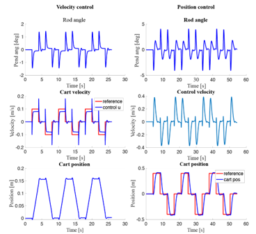
Figure 21. The pendulum angle and cart position are depicted in response to the cart movement, driven by changes in the cart position reference setpoint. Left column: MATLAB simulation of the pendulum with velocity control. The pendulum angle and cart position are shown in response to moving the cart, driven by changes in the velocity reference input. Right column: MATLAB simulation of the pendulum under position control of the cart with integral action on cart positional error.

The left column of Figure 22 shows the response of the inverted pendulum to an impulsive disturbance while operating in velocity control mode. It demonstrates a successful recovery to the initial pole deviation from the vertical position. However, it is notable that the cart position shifts and does not return to its initial starting position.

The right column of Figure 22 shows the behavior of the inverted pendulum to the same disturbance while operating in position control mode. Again it can be seen that a good recovery to the initial pole deviation from the vertical orientation is achieved. However, although the cart initially drives away from its initial location, is slowly moves back after a few seconds.

13. DIN Rail Panel Construction

13.1.           Connections to controller

A DIN rail panel was tailor-made to control the inverted pendulum system. Figures 23 and 24 show the connectors and their corresponding wiring diagrams. The controller interface, located at the top of the panel enclosure, features a female USB-B port. This port connects the Arduino Mega 2560, located inside the controller assembly, to an external computer, which is used for software development and relaying control commands.

The panel features seven female D-connectors. The interfaces are configured to connect with four stepper motors, an I²C device, an SPI device, and two encoders. The use of these D-connectors allows for easy and quick connection of the panel to the inverted pendulum apparatus or other equipment.

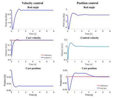
Figure 22. The pendulum angle and cart position are depicted in response to a simulated tap. Left column: MATLAB simulation of the pendulum with velocity control. The pendulum angle and cart position are shown in response to a 40 deg/s initial velocity disturbance. Right column: MATLAB simulation of the pendulum under position control of the cart, with integral action on cart positional error.

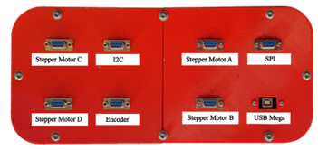
Figure 23. View of the actual controller panel cover, which was designed in Autodesk Fusion 360 and then 3D printed.

Special care was taken in the wiring of the plugs for each attached component, and they were configured with a unique connection pattern. This design feature serves to prevent accidental inappropriate connections that could result in electrical damage. The primary focus was on the power pin assignments, ensuring their isolation from other signal inputs and outputs. This safeguard ensures that potential connection errors will not result in component damage.

13.2.           Panel internal layout

The controller panel’s internal layout comprises three specific DIN rails, as depicted in Figure 25, which shows a photograph of the assembled unit. It consists of a microcontroller rail, a rail for motor drivers and power converters, and a power supply rail. Additionally, wiring conduit was strategically placed to manage the cabling in a tidy manner. This arrangement not only enhanced the orderly appearance but also reduced the risk of unintended cable contact with other components or causing interference.

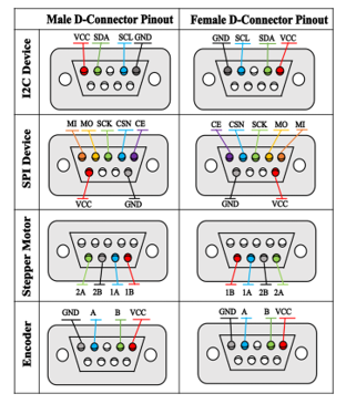
Figure 24. Rear view of soldered D-Sub connections on the male plugs (left-hand column) and the female sockets (right-hand column) mounted on the panel. The top row shows the Inter-Integrated Circuit (I²C) pinout, the second row is for Serial Peripheral Interface (SPI), the third row is dedicated to stepper motors, and the bottom row is configured for encoders

13.3.           Panel DIN rail components

In the selection of panel components, preference was given to components equipped with rear mounts for DIN rail attachment. For other components, custom 3D printed support structures were made and fitted with clips to attach them to the DIN rails. The power rail within the controller panel was compartmentalized into three principal sections:

1. An AC circuit breaker section that is responsible for regulating overcurrent conditions and interrupting the main supply.
2. A region featuring a PULS Dimension DIN rail power supply, which delivers 24 volts at 5A, and meets the voltage and current prerequisites of the system.
3. A region containing three discrete DC circuit breakers, to permit individual disconnection of each control component. This feature provides additional protection against potential damage due to short circuits.

13.4.           Stepper motor drivers

The power converter and motor driver rails were engineered to facilitate the operation of up to four stepper motors, each capable of being directly interfaced with the control panel’s motor driver rail. The motor driver rail featured two 3D-printed carriers, each housing a pair of A4988 stepper motor drivers. These motor drivers were powered by a 24-volt supply operating on mains power.

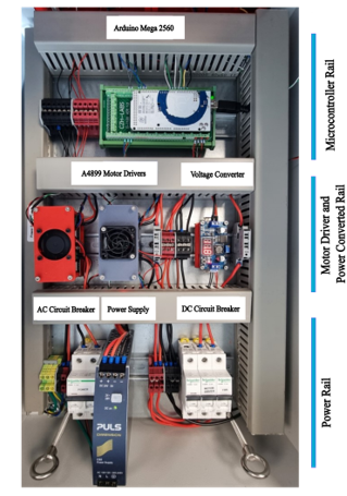
Figure 25. View displaying the internal layout of the controller panel, which is partitioned into distinct sections for power management, motor control, and microcontroller functions.

The A4988 driver offers eight distinct micro-stepping resolutions, providing flexibility in stepper motor control. For this project, we employed a one-fourth step resolution for all motors. To realize the one-fourth step resolution setting on the expansion board, the DIL switches were configured appropriately. The A4988 driver can operate within a voltage range of 8V to 35V and can deliver a current ranging from 1.5A to 2.2A. A potentiometer is incorporated into the driver breakout board, enabling hands-on fine-tuning of the current supplied to the stepper motor. To determine the current limit, I_lim, it’s essential to gauge the reference voltage (V_ref) on the potentiometer and apply the given formula to compute its desired value:

This facilitates precise control over the motor current, optimizing performance and efficiency. Our adjustment of the current limit was a critical step to ensure the proper functioning of our NEMA23 stepper motors. A current limit of 1.5A was determined to be ideal for this specific application. Exceeding this current threshold may damage both the motors and the drivers. Conversely, setting the current below 1.5A could compromise the motors’ operation, raising the likelihood of stalling. Thus, appropriate calibration is paramount to ensure good performance while safeguarding the components from potential harm.

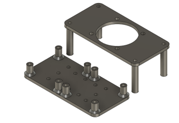
Figure 26. DIN Rail holder for the A4988 Driver Module. This setup mounts two stepper motor controller breakout boards onto a DIN rail. Notably, it includes a cooling fan to ensure the controllers remain at optimal temperatures and prevent overheating.

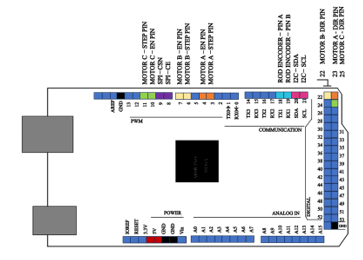
Figure 27. Pinouts for the Arduino Mega 2560. The connections are configured to control up to three stepper motors and communicate with peripherals via the I²C and SPI data buses.

To prevent overheating of the motor drivers, the incorporation of a cooling solution was essential. A pair of compact DC axial fans were positioned above them to prevent thermal damage to the chips. These fans required a supply voltage of 12V, which was furnished through a Buck converter operating from the 24V power line (refer to Figure 26). This setup ensured that the motor drivers stayed at a safe temperature during operation, enhancing both their performance and longevity.

At the heart of the controller panel, on the microcontroller rail, the Arduino Mega 2560 is prominently featured. Selected for its robust I/O capabilities, it offers 54 digital input/output pins, including 15 suitable for PWM, 256KB of flash memory, and a clock speed of 16MHz (refer to Figures 27 and 28). The Arduino Mega facilitates seamless communication with the host PC, aligning perfectly with the project’s requirements.

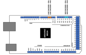
Figure 28. Arduino Mega 2560 pinout connections used for reading the system’s two encoders.

14. Software Implementation in Arduino

14.1.           Arduino software overview

Control over the pendulum was overseen by the Arduino Mega, which was employed to implement a state feedback controller function within its primary polling loop. During the polling operation, the control process begins by reading the encoder to ascertain the pendulum pole’s angle relative to the vertical. For the state feedback controller to operate, it required the pendulum system’s full state. Since only the angle was directly available, the second state was estimated using a Luenberger observer. Using the full state estimate, the control command was generated by multiplying it with the specified feedback gain. Based on the measured angle, the feedback controller then calculated the stepper motor velocity control signal. This signal produced an output pulse train, driving the stepper motor and allowing the cart to move at the ideal speed to maintain balance. State updates were computed utilizing Euler integration.

14.2.           Arduino command menu

Within the polling cycle, the system processes and interprets incoming commands received through the serial interface. The suite of accessible commands encompasses the following:

• Activate control: Starts balancing when the pendulum is brought up to an inverted configuration.
• Deactivate control.
• Display help menu: View controller parameters.

14.3.           Main Arduino loop pseudocode

The pseudocode for the main Arduino poll loop is shown below. This makes use of function calls the can reset the encoder, calculate the motor command, and drive the stepper motor. The loop is continuously run to control the system, ensuring that the pendulum maintains its desired position or follows a certain trajectory. In addition, there are command responses from calls to the menu system so that the program can be operated from a serial monitor over a USB connection.

Main Arduino Poll loop
Result: Balances pendulum on track
Initialization of SFC parameters and flags
while program running do
	Call the menu object for input commands, act accordingly Read time Read pendulum pole angle Read reference value Call SFC function to compute control u Generate stepper control pulses to Drive stepper motor
end

14.4.           Pseudocode to implement SFC

The state feedback controller is implemented as a C++ class. Its constructor sets up the parameters for the state space model, as well as the SFC gain K and the Luenberger gain L. A SFC function is called with the current time and the measured pendulum pole position. It returns the control value U, which is subsequently used to set the rotational velocity of the stepper motor and drive the pendulum cart.

State Feedback Controller
Result: state feedback control variable u
Initialization state space matrices A, B, C Initialization SFC gain K Initialization Luenberger gain L Initialization state estimate;    = [0; 0; 0; 0];
while balancing pendulum do
	Read reference value ref
	Read pendulum output angle y
	Calculate time step: h. = time – lastTime
	Update last time:  lastTime = time
	Calculate control:  u = – K  + ref *
	Calculate Output prediction error: yErr = y – C
	Calculate 1st pendulum state derivative: A[0][0] * + A[0][1] * + B[0] * u + L[0] * yErr
	Calculate 2nd pendulum state derivative: A[1][0] * + A[1][1] * + B[1] * u + L[1] * yErr
	Calculate 3rd cart position state derivative: B[2] * u
	Calculate 4th integral position error state derivative: B[2] – ref
	Perform Euler integration: =  + h
	Return u
end

15. Experimental results

15.1.  Online demonstration videos

Viewers can watch the inverted pendulum operations, including various tests, on the YouTube channel ‘Robotics, Control and Machine Learning’. All related videos are grouped under the ‘ASTESJ Inverted Pendulum’ playlist. Please follow the provided link for direct access to these videos:

15.2. Perturbation tests

We use a straightforward approach to assess control law performance by simultaneously monitoring the cart’s position and the pendulum’s angle during minor system disturbances. We obtain these measurements using encoders on the cart’s stepper motor and at the pendulum’s axis for angle measurement. During the balance test, disturbances are introduced by systematically applying an impulse to the pendulum using a tapping mechanism.

Experiments were conducted in both position and velocity control modes, varying the pole length from shorter to longer dimensions. These tests demonstrated the system’s ability to maintain stability, even when subjected to additional loads altering its dynamic characteristics. Video demonstrations of these experiments can be found on YouTube, as per the link provided above.

15.3. Position mode results

Figure 29 shows the results of the test conducted in position control mode. The pendulum was initially stabilized and held stationary in a balanced position. Following the disturbance, immediate and noticeable changes occurred in both the pendulum angle and the cart’s position. The pendulum angle plot showed minor fluctuations around zero. The motor encoder data revealed that the cart moved quickly to restore balance in the system and then gradually returned to its original position. This behavior, referring to the cart’s movement and pendulum stabilization, is also evident in the YouTube videos.

During tests with the long-length pole, we observed a small oscillation of the cart, even in the absence of disturbance. This oscillation likely stems from a significant mismatch between the long-length pole’s parameters and those of the medium-length pole, for which the controller was originally designed. Based on these observations, modifying the control law appears necessary to effectively manage the pendulum’s behavior with its increased length.

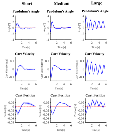
Figure 29. Responses of real, physically position-controlled inverted pendulums (using integral action on cart position) to impulsive disturbances delivered by the tapping mechanism. Results are for all three pendulum lengths in their low damping configurations. The solid blue line represents the mean response averaged across eight aligned recordings, and the light blue shading indicates the corresponding standard deviation.

15.4.  Velocity mode results

The pendulum’s performance was closely examined while operating under velocity control, as illustrated in Figure 30. The velocity control operation was initiated via the keyboard on the main PC. Users could select a cart velocity, resulting in the cart moving as specified in both left and right directions.

To further evaluate the system’s resilience against knocks, representing impulsive disturbances, we conducted an additional test. In this test, the pole was gently tapped while the velocity was set to zero. In all instances, the pendulum system demonstrated notable stability and effectiveness in mitigating the disturbance. Compared to the position control mode, disturbances in the velocity control mode led to uncompensated cart movements, particularly for the short pendulum, as shown in the lowest row of Figure 30. Again, this behavior is also apparent in the YouTube videos. This is also worth noting that using a longer pole again resulted in a modest reduction in performance in velocity control mode, with some cart oscillations observed after the impulsive disturbance. However, this effect was less pronounced than in position control mode.

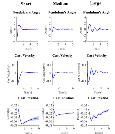
Figure 30. Responses of  real, physically velocity-controlled inverted pendulums to impulsive disturbances delivered by the tapping mechanism. Results are for all three pendulum lengths in their low damping configurations. The solid blue line represents the mean response averaged across eight aligned recordings, and the light blue shading indicates the corresponding standard deviation.

16. Discussion

16.1.  Summary

In this study, we demonstrated the design, implementation, analysis, simulation, and testing of an inverted pendulum. The mechanical system was built utilizing V-slot rail components and custom 3D printed parts.

Novel features of this work included:

1. The construction of a physical pendulum in which the pole length, viscosity, and resistive friction could be easily modified.
2. The construction of a testing rig, designed to apply consistent taps to the pendulum pole, to evaluate its reaction to impulsive disturbances.
3. Use of system identification to investigate and quantify the pendulum’s uncontrolled dynamics as the physical characteristics of the pendulum system were changed.
4. The design of two linear controllers, based on observer-based full state feedback control modes, supporting either velocity or position control of the pendulum cart while balancing the pendulum pole.
5. Performance testing to investigate the pendulum’s controlled dynamics as its physical characteristics were changed.

16.2. Uncontrolled pendulum oscillations

We first investigated the behavior of the pendulum in its stable downward inverted configurations. This was done for all three test pendulum pole lengths, as well as under conditions of both high and low static friction and high and low viscous damping. We examined the pendulum’s free oscillations following an initial large angle displacement of approximately 90°, and also after initial small angle displacements of about 5°, caused by taps from the tapping mechanism. As expected, increasing the pole length reduced the oscillatory frequency of the pendulum.

Increasing viscosity using the paddle mechanism significantly reduced the decay time of oscillations in the large angle case. In this scenario, the added viscous resistance dominated the pendulum’s oscillatory decay, resulting in an exponential reduction in amplitude over time. However, in the small angle condition, where static sliding friction was a significant source of decay, the paddle had minimal effect. This was evidenced by a more linear decay of oscillatory amplitude.

When we increased static friction equally in both the large and small angle cases, the effects differed. In the large angle case, this increase led to a noticeable, albeit modestly more linear, decay of oscillations. Conversely, in the small angle condition, the same level of friction had a dramatic effect, rapidly decelerating oscillations and bringing them to a standstill within just a few cycles.

These observations indicate that the viscous resistance from the paddle is better represented by the square of the movement velocity than by the linear model commonly used in mathematical modeling. This is particularly true since the paddle’s effect is significant only during faster movements. Furthermore, at small amplitudes, where the effect of gravity acting on the pole produces minimal torque, any substantial static frictional resistance can dominate the damping behavior.

16.3.  System identification

To estimate the pendulums’ parameters, we applied a system identification procedure to the small angle dataset. This data best represents the small angle condition occurring during the balancing of the inverted pendulum. We used optimization to fit the predicted pendulum damped oscillatory decay waveform with data recorded from the pendulum in different configurations. We noted that including a friction term in the mathematical model of the non-inverted pendulum was necessary in this process. This addition accounts for the linear aspect of decay and achieves a good fit. The fitting procedure enabled the estimation of the viscous and static friction terms, as well as an updated estimate of the effective pendulum pole length, mass, and moment of inertia.

16.4. Controlled pendulum results

We undertook a sequence of system tests, starting with the standard pendulum pole length for which the controllers were developed. We then investigated how the stabilized pendulum pole responded to light taps from the tapper mechanism, creating impulses. This testing was carried out in both velocity and position control modes. In velocity mode, the cart could be driven with a feedforward velocity command to move left or right while maintaining balance. In position control mode, which operates with integral action on the cart’s position, the control system maintains the pendulum’s cart at a specified location. We observed distinct behavioral differences between the two control modes.

Unsurprisingly, velocity control, unconcerned with cart position, responded to disturbances to the pendulum pole with balancing movements of the cart, typically causing a positional shift. In position control mode, a disturbance similarly resulted in balancing movement, but the cart gradually returned to its initial position.

Since the cart’s movement velocity is limited, any disturbance requiring faster movement would naturally result in a loss of balance. This limitation also affects the balancing robustness in velocity control mode. If the cart is already moving in one direction, its capacity for additional corrective velocity in that direction is restricted.

16.5.  Transfer of controller operation to other pole lengths

To assess controller performance, we conducted balancing system tests using both shorter and longer pendulum pole lengths, comparing them to the standard length for which the controllers were developed. We found that the controllers operated well with the shorter length pendulum pole. However, with the longer pendulum pole, we observed some oscillatory behavior of the cart, particularly in position control mode. Despite this, the inverted pendulum balance was still maintained.

We note that the gains for both controller modes, derived from the Linear Quadratic Regulator (LQR) design process, were based solely on experimentation with the standard pendulum. Naturally, there remains a strong likelihood that more optimal controllers for both modes could exist, particularly if they were specifically designed for these varying pendulum lengths.

16.6.  Future work

In the current study, we examined the effects of a relatively low-intensity, fixed impulsive disturbance on pendulums using a tapper mechanism. We utilized this setup to assess how the pendulums responded as their characteristics were altered and to observe the behaviors of velocity and position control. These tests did not result in a loss of balance; rather, they only evaluated the reactions necessary to maintain equilibrium. It would be enlightening to apply a wider range of impulse intensities and compare the behaviors related to loss of balance across the various conditions and controllers examined in this study. The existing tapper mechanism could not be easily adjusted to provide a range of impulse intensities. For future research, constructing a tapper device that employs a motor to drive the tapper rod would be a valuable exercise, allowing for precise control over the impulse intensity.

Currently, we have examined the behavior of two different state feedback controller architectures for balancing a pendulum. Many other control approaches exist, and a comparison with methods such as PID (Proportional-Integral-Derivative) [16,17],  and reinforcement learning [22–24], would be informative.

The inverted pendulum has been valuable in understanding human balance while standing [44–52]. Future studies within the framework of our pendulum system could further explore and model human behavior in such tasks. These studies could investigate factors that constrain human performance, including sensory feedback latency, noise in the control and sensory systems, as well as the force, stiffness, and speed of movement characteristics of muscles [68]. Such issues could be readily incorporated into the MATLAB simulations as well as real-time control of the physical pendulum system.

Conflict of Interest

The authors declare no conflict of interest.

Acknowledgment

Support for LAH was provided by the Engineering and Physical Sciences Research Council and The University of Plymouth. ISH was supported by The University of Plymouth. We also thank Jonathan Marsden and Gunnar Schmidtmann in the School of Health Professions at the University of Plymouth, for insightful discussions on this work.

1. L. Alvarez-Hidalgo, I.S. Howard, “Gain scheduling for state space control of a dual-mode inverted pendulum,” in 2022 International Conference on System Science and Engineering (ICSSE), IEEE: 39–46, 2022, doi:10.1109/ICSSE55923.2022.9947361.
2. P. Horáček, “Laboratory experiments for control theory courses: A survey,” Annual Reviews in Control, 24, 151–162, 2000, doi:https://doi.org/10.1016/S1367-5788(00)90029-4.
3. K.H. Lundberg, T.W. Barton, “History of inverted-pendulum systems,” IFAC Proceedings Volumes, 42(24), 131–135, 2010, doi:https://doi.org/10.3182/20091021-3-JP-2009.00025.
4. H. Wang, H. Dong, L. He, Y. Shi, Y. Zhang, “Design and simulation of LQR controller with the linear inverted pendulum,” in 2010 international conference on electrical and control engineering, IEEE: 699–702, 2010, doi: 10.1109/iCECE.2010.178.
5. I. Kafetzis, L. Moysis, “Inverted Pendulum: A system with innumerable applications,” School of Mathematical Sciences, 2017.
6. O. Boubaker, “The inverted pendulum benchmark in nonlinear control theory: a survey,” International Journal of Advanced Robotic Systems, 10(5), 233, 2013, doi:https://doi.org/10.5772/55058.
7. N. Muskinja, B. Tovornik, “Swinging up and stabilization of a real inverted pendulum,” IEEE Transactions on Industrial Electronics, 53(2), 631–639, 2006, doi:10.1109/TIE.2006.870667.
8. M. Turner, T.R. Cooley, “A Low-cost and Flexible Open-source Inverted Pendulum for Feedback Control Laboratory Courses,” in 2015 ASEE Annual Conference & Exposition, 26.63. 1-26.63. 13, 2015, doi:DOI:10.18260/p.23404.
9. K. Kaheman, U. Fasel, J.J. Bramburger, B. Strom, J.N. Kutz, S.L. Brunton, “The experimental multi-arm pendulum on a cart: A benchmark system for chaos, learning, and control,” ArXiv Preprint ArXiv:2205.06231, 2022, doi:https://doi.org/10.48550/arXiv.2205.06231.
10. F. Grasser, A. D’arrigo, S. Colombi, A.C. Rufer, “JOE: a mobile, inverted pendulum,” IEEE Transactions on Industrial Electronics, 49(1), 107–114, 2002, doi:10.1109/41.982254.
11. H. Vasudevan, A.M. Dollar, J.B. Morrell, “Design for control of wheeled inverted pendulum platforms,” Journal of Mechanisms and Robotics, 7(4), 41005, 2015, doi:https://doi.org/10.1115/1.4029401.
12. M. Hehn, R. D’Andrea, “A flying inverted pendulum,” in 2011 IEEE International Conference on Robotics and Automation, IEEE: 763–770, 2011, doi:10.1109/ICRA.2011.5980244.
13. S. Awtar, N. King, T. Allen, I. Bang, M. Hagan, D. Skidmore, K. Craig, “Inverted pendulum systems: rotary and arm-driven-a mechatronic system design case study,” Mechatronics, 12(2), 357–370, 2002, doi:https://doi.org/10.1016/S0957-4158(01)00075-7.
14. B. Tomar, N. Kumar, M. Sreejeth, “Optimal Control of Rotary Inverted Pendulum Using Continuous Linear Quadratic Gaussian (LQG) Controller,” in 2023 14th International Conference on Computing Communication and Networking Technologies (ICCCNT), IEEE: 1–6, 2023, doi:10.1109/ICCCNT56998.2023.10306449.
15. P. Strakoš, J. Tůma, “Mathematical modelling and controller design of inverted pendulum,” in 2017 18th International Carpathian Control Conference (ICCC), IEEE: 388–393, 2017, doi:10.1109/CarpathianCC.2017.7970431.
16. Sultan, A. Mirza, “Inverted Pendulum, Analysis, Design and Implementation,” Visionaries Document, 2003.
17. Razzaghi, A.A. Jalali, “A new approach on stabilization control of an inverted pendulum, using PID controller,” Advanced Materials Research, 403, 4674–4680, 2012, doi:https://doi.org/10.4028/www.scientific.net/AMR.403-408.4674.
18. S. Howard, “A modular 3D-printed inverted pendulum,” in Towards Autonomous Robotic Systems: 20th Annual Conference, TAROS 2019, London, UK, July 3–5, 2019, Proceedings, Part I 20, Springer: 413–424, 2019, doi:https://doi.org/10.1007/978-3-030-23807-0_34.
19. A. Ibanez, O.G. Frias, M.S. Castanon, “Lyapunov-based controller for the inverted pendulum cart system,” Nonlinear Dynamics, 40, 367–374, 2005, doi:https://doi.org/10.1007/s11071-005-7290-y.
20. Yang, P. Wang, T. Zhang, “Modelling and controller design of planar inverted pendulum system,” in 2014 International Conference on Mechatronics, Electronic, Industrial and Control Engineering (MEIC-14), Atlantis Press: 57–61, 2014, doi:10.2991/meic-14.2014.14.
21. Lipson, Robots on the run, 2019, doi:doi: https://doi.org/10.1038/d41586-019-00999-w.
22. Safeea, P. Neto, “A Q-learning approach to the continuous control problem of robot inverted pendulum balancing,” Intelligent Systems with Applications, 200313, 2023, doi:https://doi.org/10.1016/j.iswa.2023.200313.
23. Ma, D. Xu, J. Huang, Y. Li, “Robust Control of An Inverted Pendulum System Based on Policy Iteration in Reinforcement Learning,” Applied Sciences, 13(24), 13181, 2023, doi:https://doi.org/10.3390/app132413181.
24. Israilov, L. Fu, J. Sánchez-Rodríguez, F. Fusco, G. Allibert, C. Raufaste, M. Argentina, “Reinforcement learning approach to control an inverted pendulum: A general framework for educational purposes,” PLoS One, 18(2), e0280071, 2023, doi:https://doi.org/10.1371/journal.pone.0280071.
25. Deisenroth, C.E. Rasmussen, “PILCO: A model-based and data-efficient approach to policy search,” in Proceedings of the 28th International Conference on machine learning (ICML-11), 465–472, 2011.
26. W. Anderson, “Learning to control an inverted pendulum using neural networks,” IEEE Control Systems Magazine, 9(3), 31–37, 1989, doi:10.1109/37.24809.
27. Mladenov, G. Tsenov, L. Ekonomou, N. Harkiolakis, P. Karampelas, “Neural network control of an inverted pendulum on a cart,” in WSEAS International Conference. Proceedings. Mathematics and Computers in Science and Engineering, World Scientific and Engineering Academy and Society, 2009.
28. Suresh, M.P.F. Queen, V.A.T.P. Symon, A. Linsely, “Control and stabilization of inverted pendulum using GA based controller,” International Journal of Mechanical Engineering and Technology, 8(8), 748–756, 2017.
29. Omatu, S. Deris, “Stabilization of inverted pendulum by the genetic algorithm,” in Proceedings of IEEE international conference on evolutionary computation, IEEE: 700–705, 1996, doi:10.1109/ICEC.1996.542687.
30. S. Sazonov, P. Klinkhachorn, R.L. Klein, “Hybrid LQG-neural controller for inverted pendulum system,” in Proceedings of the 35th Southeastern Symposium on System Theory, 2003., IEEE: 206–210, 2003, doi:10.1109/SSST.2003.1194559.
31. Kumar, K. Chakraborty, R.R. Mukherjee, S. Mukherjee, “Modelling and controller design of inverted pendulum,” International Journal of Advanced Research in Computer Engineering & Technology (IJARCET), 2(1), 2013.
32. Zhong, H. Rock, “Energy and passivity based control of the double inverted pendulum on a cart,” in Proceedings of the 2001 IEEE International Conference on Control Applications (CCA’01)(Cat. No. 01CH37204), IEEE: 896–901, 2001, doi:10.1109/CCA.2001.973983.
33. Baek, C. Lee, Y.S. Lee, S. Jeon, S. Han, “Reinforcement learning to achieve real-time control of triple inverted pendulum,” Engineering Applications of Artificial Intelligence, 128, 107518, 2024, doi:https://doi.org/10.1016/j.engappai.2023.107518.
34. An, Y. Li, “Simulation and control of a two-wheeled self-balancing robot,” in 2013 IEEE International Conference on Robotics and Biomimetics (ROBIO), IEEE: 456–461, 2013, doi:DOI: 10.1109/ROBIO.2013.6739501.
35. Hasan, C. Saha, M.M. Rahman, M.R.I. Sarker, S.K. Aditya, “Balancing of an inverted pendulum using PD controller,” Dhaka University Journal of Science, 60(1), 115–120, 2012, doi:DOI: 10.3329/dujs.v60i1.10348.
36. -S. Juang, K.-Y. Lum, “Design and control of a two-wheel self-balancing robot using the arduino microcontroller board,” in 2013 10th IEEE International Conference on Control and Automation (ICCA), IEEE: 634–639, 2013, doi:DOI: 10.1109/ICCA.2013.6565146.
37. Wang, L. Cui, J. Zhang, J. Lai, D. Zhang, K. Chen, Y. Zheng, Z. Zhang, Z.-P. Jiang, “Balance control of a novel wheel-legged robot: Design and experiments,” in 2021 IEEE International Conference on Robotics and Automation (ICRA), IEEE: 6782–6788, 2021, doi:10.1109/ICRA48506.2021.9561579.
38. Darvish, L. Penco, J. Ramos, R. Cisneros, J. Pratt, E. Yoshida, S. Ivaldi, D. Pucci, “Teleoperation of humanoid robots: A survey,” IEEE Transactions on Robotics, 2023, doi:10.1109/TRO.2023.3236952.
39. Bratta, M. Focchi, N. Rathod, C. Semini, “Optimization-Based Reference Generator for Nonlinear Model Predictive Control of Legged Robots,” Robotics, 12(1), 6, 2023, doi:https://doi.org/10.3390/robotics12010006.
40. A. Castano, J. Humphreys, E. Mingo Hoffman, N. Fernández Talavera, M.C. Rodriguez Sanchez, C. Zhou, “Benchmarking Dynamic Balancing Controllers for Humanoid Robots,” Robotics, 11(5), 114, 2022, doi:https://doi.org/10.3390/robotics11050114.
41. Kajita, M. Morisawa, K. Miura, S. Nakaoka, K. Harada, K. Kaneko, F. Kanehiro, K. Yokoi, “Biped walking stabilization based on linear inverted pendulum tracking,” in 2010 IEEE/RSJ International Conference on Intelligent Robots and Systems, IEEE: 4489–4496, 2010, doi:10.1109/IROS.2010.5651082.
42. A. Winter, “Human balance and posture control during standing and walking,” Gait & Posture, 3(4), 193–214, 1995, doi:https://doi.org/10.1016/0966-6362(96)82849-9.
43. Quijoux, A. Nicolaï, I. Chairi, I. Bargiotas, D. Ricard, A. Yelnik, L. Oudre, F. Bertin‐Hugault, P. Vidal, N. Vayatis, “A review of center of pressure (COP) variables to quantify standing balance in elderly people: Algorithms and open‐access code,” Physiological Reports, 9(22), e15067, 2021, doi:https://doi.org/10.14814/phy2.15067.
44. Gawthrop, I. Loram, M. Lakie, H. Gollee, “Intermittent control: a computational theory of human control,” Biological Cybernetics, 104, 31–51, 2011, doi:https://doi.org/10.1007/s00422-010-0416-4.
45. D. Loram, H. Gollee, C. van de Kamp, P.J. Gawthrop, “Is Intermittent Control the Source of the Non-Linear Oscillatory Component (0.2–2Hz) in Human Balance Control?,” IEEE Transactions on Biomedical Engineering, 69(12), 3623–3634, 2022, doi:10.1109/TBME.2022.3174927.
46. G. Milton, “Time delays and the control of biological systems: An overview,” IFAC-PapersOnLine, 48(12), 87–92, 2015.
47. Milton, J.L. Cabrera, T. Ohira, S. Tajima, Y. Tonosaki, C.W. Eurich, S.A. Campbell, “The time-delayed inverted pendulum: implications for human balance control,” Chaos: An Interdisciplinary Journal of Nonlinear Science, 19(2), 2009, doi:https://doi.org/10.1063/1.3141429.
48. Kot, A. Nawrocka, “Modeling of human balance as an inverted pendulum,” in Proceedings of the 2014 15th International Carpathian Control Conference (ICCC), IEEE: 254–257, 2014, doi:10.1109/CarpathianCC.2014.6843607.
49. D. Loram, M. Lakie, “Human balancing of an inverted pendulum: position control by small, ballistic‐like, throw and catch movements,” The Journal of Physiology, 540(3), 1111–1124, 2002, doi:https://doi.org/10.1113/jphysiol.2001.013077.
50. -L. Sung, C.-Y. Hong, C.-H. Liu, P. Lee, L.-Y. Guo, N.-H. Lin, C.-W. Yen, L.-J. Liaw, “Characterizing the validity of the inverted pendulum model for quiet standing,” Journal of Healthcare Engineering, 2021, 1–6, 2021, doi:https://doi.org/10.1155/2021/8884614.
51. D. Loram, H. Gollee, M. Lakie, P.J. Gawthrop, “Human control of an inverted pendulum: is continuous control necessary? Is intermittent control effective? Is intermittent control physiological?,” The Journal of Physiology, 589(2), 307–324, 2011, doi:https://doi.org/10.1113/jphysiol.2010.194712.
52. Morasso, A. Cherif, J. Zenzeri, “Quiet standing: The single inverted pendulum model is not so bad after all,” PLoS One, 14(3), e0213870, 2019, doi:https://doi.org/10.1371/journal.pone.0213870.
53. Franklin, J. Česonis, D.W. Franklin, “Influence of visual feedback on the sensorimotor control of an inverted pendulum,” in 2018 40th Annual International Conference of the IEEE Engineering in Medicine and Biology Society (EMBC), IEEE: 5170–5173, 2018, doi:10.1109/EMBC.2018.8513461.
54. Česonis, S. Franklin, D.W. Franklin, “A simulated inverted pendulum to investigate human sensorimotor control,” in 2018 40th Annual International Conference of the IEEE Engineering in Medicine and Biology Society (EMBC), IEEE: 5166–5169, 2018, doi:10.1109/EMBC.2018.8513434.
55. Leib, J. Česonis, S. Franklin, D.W. Franklin, “LQG framework explains performance of balancing inverted pendulum with incongruent visual feedback,” in 2019 41st Annual International Conference of the IEEE Engineering in Medicine and Biology Society (EMBC), IEEE: 1940–1943, 2019.
56. Franklin, J. Česonis, R. Leib, D.W. Franklin, “Feedback delay changes the control of an inverted pendulum,” in 2019 41st Annual International Conference of the IEEE Engineering in Medicine and Biology Society (EMBC), IEEE: 1517–1520, 2019, doi:10.1109/EMBC.2019.8856897.
57. Ghorbani, M.A. Shooredeli, M. Teshnehlab, “Fault tolerant improvement with chaos synchronization using Fuzzy-PID control,” in 2013 13th Iranian Conference on Fuzzy Systems (IFSC), IEEE: 1–5, 2013, doi:10.1109/IFSC.2013.6675645.
58. F. Hamza, H.J. Yap, I.A. Choudhury, A.I. Isa, A.Y. Zimit, T. Kumbasar, “Current development on using Rotary Inverted Pendulum as a benchmark for testing linear and nonlinear control algorithms,” Mechanical Systems and Signal Processing, 116, 347–369, 2019, doi:https://doi.org/10.1016/j.ymssp.2018.06.054.
59. H. Raibert, H.B. Brown Jr, “Experiments in balance with a 2D one-legged hopping machine,” 1984, doi:https://doi.org/10.1115/1.3149668.
60. -S. Juang, K.-Y. Lum, “Design and control of a two-wheel self-balancing robot using the arduino microcontroller board,” in 2013 10th IEEE International Conference on Control and Automation (ICCA), IEEE: 634–639, 2013.
61. Monteleone, F. Negrello, G. Grioli, M.G. Catalano, A. Bicchi, M. Garabini, “A method to benchmark the balance resilience of robots,” Frontiers in Robotics and AI, 9, 2022, doi:https://doi.org/10.3389/frobt.2022.817870.
62. C. Simbach, J. Priest, “Another look at a damped physical pendulum,” American Journal of Physics, 73(11), 1079–1080, 2005, doi:http://dx.doi.org/10.1119/1.1858488.
63. F. da C. Zonetti, A.S.S. Camargo, J. Sartori, D.F. De Sousa, L.A. de O. Nunes, “A demonstration of dry and viscous damping of an oscillating pendulum,” European Journal of Physics, 20(2), 85, 1999, doi:DOI: 10.1088/0143-0807/20/2/004.
64. R. Lapidus, “Motion of a harmonic oscillator with sliding friction,” Am. J. Phys, 38(11), 1360–1361, 1970, doi: http://dx.doi.org/10.1119/1.1976111.
65. I. Molina, “Exponential versus linear amplitude decay in damped oscillators,” The Physics Teacher, 42(8), 485–487, 2004, doi:http://dx.doi.org/10.1119/1.1814324.
66. J. Åström, R.M. Murray, Feedback systems: an introduction for scientists and engineers, Princeton university press, 2021.
67. B. Moler, Numerical computing with MATLAB, SIAM, 2004.
68. W. Franklin, D.M. Wolpert, “Computational mechanisms of sensorimotor control,” Neuron, 72(3), 425–442, 2011, doi:10.1016/j.neuron.2011.10.006.

(Click Here)