The First Study on Ionospheric Peak Variability over Equatorial Africa (COSMIC-2)
 , Obiageli Josphine Ugonabo, Tafon Williams Sivla, Akor John Yakubu, Eucheria Chidinma Okoro
Adv. Sci. Technol. Eng. Syst. J. 10(4), 14–19 (2025);
 DOI: 10.25046/aj100402
In regions like the African equatorial region, where ground-based sensors like ionosondes and incoherent scatter radars are limited, satellite-based radio occultation (RO) observations offer a new alternative for ionospheric data collecting and optimization. Using RO measurements from the mostly newly launched COSMIC-2 (Constellation Observing System for Meteorology, Ionosphere, and Climate-2) mission, hence, the equatorial Africa, ionospheric peak parameters were first studied and published. Data obtained over Ilorin (8.50oN, 4.50oE) and Abuja (8.99oN, 7.38oE) from October 2019 to December 2020 were utilized in this study. The results show that diurnal profiles of NmF2 and hmF2 have crests at around 10:00 to 18:00 UT and troughs at around 04:00 to 05:00 UT. The NmF2 values are usually less than 2×105 cm-3 during the early morning hours before sunrise, and they can reach~ 6-10 ×105 cm-3 after sunrise, depending on season. NmF2 and hmF2 exhibit peaks between 18:00 UT and 10:00 UT and troughs between 05:00 UT and 04:00 UT. For the seasonal variation, the NmF2 values can reach approximately 6–10 ×105 cm-3 after sunrise, while they are often less than 2×105 cm-3 in the early morning hours before sunrise. We recorded higher values in the equinoxes (March and September) season than in the solstices (June and December) season. The 2016-IRI model overestimates the COSMIC-2 NmF2 measurements, typically during the decline phases of the 24-hour trend at 60% differences. During the March equinox season, the percentage RMSD (root-mean-squared deviation) is (~ 29%) smaller than the solstice seasons with (~30%). The percentage RMSD (root-mean-squared deviation) is the smallest. The disparity was so much observed during the September equinox, at a time when RMSD reaches ~ 1.7×10⁵ electrons/cm3 and the percentage RMSD reaches ~ 35%.
1. Introduction
The ionosphere is a region with the highest ionization in the Earth’s atmosphere. It is identified as the upper part of the Earth’s atmosphere in which free electrons and ions exist under the control of the gravity and magnetic field of the planet, and whose concentration is sufficient to affect the propagation of electromagnetic waves [1] and [2]. This region of the Earth’s atmosphere extends from roughly 60 kilometers to 1000 kilometers in height [3]. It includes the mesosphere, thermosphere, and a portion of the exosphere [4]. Due to its electrification attribute, the ionosphere interacts and influences radio propagation through it [5]. Because the upper atmosphere and upper ionosphere are co-located, the very high temperatures in the upper atmosphere persist in the upper ionosphere, which is a result of X-ray radiation from the Sun [6]. According to some researchers [7], [8], [9], [10] and [11]. Ionosphere is said to be critical and essential in telecommunication because it allows radio waves to travel both short and long distances on Earth. It also affects has been studied extensively using different satellite-based and ground-based technologies. Ionosondes/digisondes are one of the most reliable sources of ionospheric electron density (edensity) information. However, in the African equatorial region due to relatively high costs of installation and maintenance the mentioned instrument for measuring ionosphere is unavailable. Satellite-based systems, like the COSMIC (Constellation Observing System for Meteorology, Ionosphere, and Climate) mission, offer good opportunities to acquire ionospheric density information over the African equatorial region through radio occultation (RO) technique. The technique has the advantages of global coverage, high vertical resolution, and the absence of signal disturbances caused by the troposphere [12]. When a low-Earth orbit receiver (like the COSMIC satellite) observes a rising or setting GNSS satellite, a GNSS-RO takes place [13]. Because atmospheric refractivity modifies the occulted GNSS signals, this signal is examined to provide data on ionospheric electron density and other atmospheric parameters like density, pressure, temperature and humidity [14], [15] and [16].
The RO technique was first demonstrated with the GPS/MET experiment [17] and [18] and its success has led to applying the technique in many more satellite missions, including the COSMIC mission. Several authors have used the COSMIC data such as [19], [20], [21] and [22] to study the variation of ionospheric electron distribution in various parts of the globe. The peak value of edensity, NmF2, and the corresponding height of peak edensity, hmF2, do characterize electron density distribution in the ionosphere, and they are therefore key parameters for modeling the edensity distribution in the ionosphere. The COSMIC satellites are low-earth orbiting satellites with an altitudinal resolution. It varies depending on the specific implementation and instrumentation, but it is typically on the order of 0.5-1.4 kilometers (0.3-0.9 miles) [23]. These studies were based on the total electron content (TEC) parameter integrated from the COSMIC-2 measurements. There is a particularly lacking research report on the behavior of RO-derived density measurements in the African equatorial region, and much more, using the newly launched COSMIC-2 mission measurements. These kinds of studies are necessary to provide scientists/researchers with vital information on the performance of such measurements. The purpose of this research is to use RO density measurements obtained from the COSMIC-2 mission to characterize the ionospheric edensity in the equatorial African region. This is the first study employing RO electron density measurements from the COSMIC-2 mission to characterize the African equatorial ionosphere.
2. Data and Methods
Data was obtained from the University Corporation for Atmospheric Research (https://data.cosmic.ucar.edu/gnss-ro/) in the form of ionPrf files (second-level processed files). Data is available on this website starting from the 1st of October 2019. All available data from the 1st of October 2019 to the 7th of December 2020 were used. Data obtained from two stations in Nigeria, specifically Abuja (8.99oN, 7.38oE) and Ilorin (8.50oN, 4.50oE) was used in this study. We considered only observations falling within a circular window of radius 5 great circle degrees around each of the stations. Ilorin ionosonde measurements were used for comparison with corresponding COSMIC measurements. The hourly values measurement for diurnal variabilities of NmF2 and hmF2 over the seasons for each season was calculated. The seasons were constituted as follows: March equinox (March and April), June solstice (May, June, July and August), September equinox (September and October), and December solstice (January, February, November and December) according to [24]. DST data was obtained from OmniWeb (https://omniweb.gsfc.nasa.gov/form/dx1.html) only data for geomagnetic quiet days (|DST| < 30 nT) was used for this computation.
The median absolute deviation (MAD) processing of the NmF2 and hmF2 variabilities expressed in equation (1) was computed as a measure of the typical deviations from the median values.
$$MAD = \operatorname{median}(|X_i – \hat{X}|) \tag{1}$$
Where are elements in the distribution, and is median of the distribution
$$RMSD = \left( \frac{\sum_{i=1}^n (C_i – I_i)^2}{n} \right)^{0.5} \tag{2}$$$
Where and are respectively corresponding COSMIC and IRI model values, and is the number of samples.
3. Results and Discussion
The results presented in this paper are in two scenarios; in the first scenario, the altitudinal variation of electron density is presented, and in the second scenario, the diurnal and seasonal variations of the NmF2 and hmF2 parameters are presented.
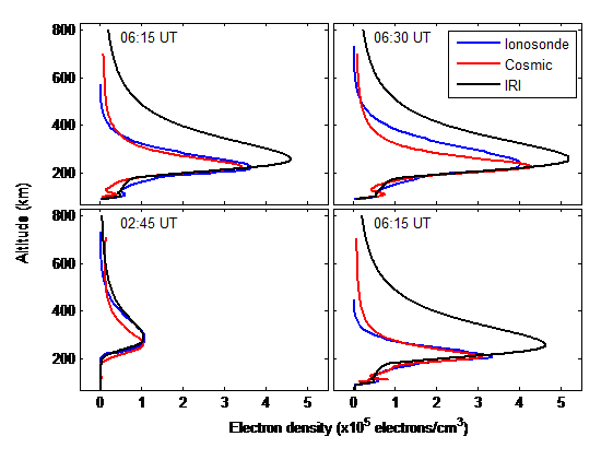
Figure1. Electron density (edensity) profiles obtained from COSMIC-2 mission, Ionosonde and 2016-IRI model for Ilorin. The edensity profiles on the top panel are respectively for 06:15 UT and 06:30 UT on day number 274 (October 1), year 2019, while the electron density profiles on the bottom panel are respectively for 02:45 UT and 06:15 UT on day number 276 (October 3), year 2019.
Figure 1 shows the altitudinal variations of edensities at four different times in two days when there was a record of coincident edensity measurements from both COSMIC and ionosonde equipment. The edensity profiles on the top panel are respectively for 06:15 UT and 06:30 UT on day number 274 (October 1), the year 2019, while the edensity profiles on the bottom panel are respectively for 02:45 UT and 06:15 UT on day number 276 (October 3), the year 2019. Local time in Nigeria is UT+1 hour. It is important to clarify here that we would have been interested to show these results from different times of the day, but we are limited by the number of times when there are coincident observations from both COSMIC and ionosonde equipment. Throughout the study investigated in this research, there was available data from the ionosonde only during the few days between days numbers 274 and 277. During these few days, coincident COSMIC measurements were recorded during the times illustrated. We considered only COSMIC measurements recorded within a spatial window of 5 great circle degrees around the Ilorin ionosonde station and within a time window of 15 minutes of the ionosonde measurement.
Figure 1 illustrates the typical pattern of electron density variation with altitude at the location. The figure shows that the edensities typically peak at about 250 – 300 km. It is evident from the figure that the IRI model overestimates the peak parameters (both the peak edensity value and the height of peak edensity), especially for the profiles around 06:15 and 06:30 UT. Panels 2 and 3 in Figure 1 provide more premises for analyzing the IRI model predictions of the peak parameters. The patterns provided by the COSMIC and ionosonde measurements are more identical, except for a case like the 02:45 UT measurement where the ionosonde measurements are slightly greater than the COSMIC measurements at around 300 – 400 km altitudes. These slight differences could be attributed to the reason that the ionosonde measurements above the F2 peak altitude are modeled values, rather than ‘pure’ measurements. The inherent modeling errors could be responsible for the slight departures noted at altitudes above the F2 peak. The good level of consistency between the ionosonde and COSMIC measurements indicates that the measurements can both be independently used to study ionospheric electron density variations in the region. Given the paucity of ionosonde data for the period of this study, we next present an extended climatologic study of the peak parameters that are based on COSMIC-2 measurements. This ionospheric variability study is the first COSMIC-2-based measurement of ionospheric peak parameters carried out in the region. Finally, the few discrepancies observed in our data between the Cosmic-2 measurement and IRI-model above the F2 peak, where the ionosonde measurement slightly overestimates Cosmic-2 densities, are attributed to the modeled nature of ionosonde outputs at those altitudes. This insight emphasizes the importance of cautious interpretation of ionsonder data above the F2 peak and supports the use of satellite-based data for capturing high altitude ionospheric structure. There was an indication that the IRI model overstatement during the early hours of (06:15 UT and 06: 30 UT). This discrepancy highlights a limitation in the IRI model’s ability to accurately capture the local ionospheric condition in equatorial West Africa. Therefore, we suggest that regional calibration of the model may be necessary to improve its performance in the zone.
Figure 2 shows diurnal variation patterns of the NmF2 at Abuja for the different seasons. For each season, hourly based median values and MADs of the NmF2 were computed as described in the Data and Methods section. In Figure 2 the NmF2 daily patterns show troughs at about 04:00 UT, just before sunrise. The figure also shows that the NmF2 values are frequently less than 2×105 cm-3 during the early morning hours before sunrise. The peaks of the diurnal NmF2 profiles are about 6-10 ×105 cm-3, and these typically occur at around 16:00 UT. The day-time values (after sunrise and before sunset) are usually greater than 4.5×105 cm-3, and the night-time values usually drop below 2×105 cm-3. Seasonally, equinoxes (March and September) have higher NmF2 values than during the solstices (June and December). This is because the location is in the equatorial region; the equatorial region receives more direct sunlight during the equinoxes than during the solstices. It is also evident from Figure 2 that there is good agreement between the NmF2 profiles produced by the IRI model and COSMIC-2. The patterns of the profiles are similar. Table 1 contains statistics on the relationship between the IRI model and COSMIC-2 profiles. The table shows that correlation coefficients between the profiles are greater than 0.9 for each of the four seasons. The values reveal that there is the greatest similarity in the patterns of the profiles during the June solstice. The IRI and COSMIC-2 NmF2 values are frequently observed to be within the error limits of each other. However, there are occasional disparities between the two datasets. Table 1 contains information on the root-mean-squared differences (RMSDs) and associated percentage differences between the two datasets. The RMSDs, computed using the formula in equation (2), are measures of the differences between the two datasets; they indicate the typical differences between the datasets in units of electron density, while the percentage difference indicates the difference as a percentage of the electron density at the given instances.

Smaller values of the RMSD and the percentage difference therefore connote better agreement between the two datasets. The table, as well as Figure 2, show that smaller RMSDs (root-mean-squared differences) are obtained during the solstice seasons (~ 1.1×10⁵ electrons/cm3). These are therefore the seasons when the IRI model values have better agreement with the COSMIC-2 measurements. The smallest RMSD is particularly recorded during the June solstice season. Considering that it is also in the June season that the two datasets have the greatest correlation, we note that the IRI model most accurately reproduces COSMIC-2 measurements during the June solstice.
Table 1: Table of correlation coefficients, RMSDs, and percentage RMSDs, computed between COSMIC-2 NmF2 measurements and IRI model values
| Season | Correlation coefficient | RMSD (×105 electrons/cm3) | Percentage RMSD (%) |
| March equinox | 0.96 | 1.23 | 29.01 |
| June solstice | 0.99 | 1.07 | 31.64 |
| September equinox | 0.95 | 1.67 | 35.78 |
| December solstice | 0.92 | 1.09 | 30.49 |
One valid argument is that the RMSDs are smaller for the solstices because the edensity magnitudes are correspondingly smaller for the solstice seasons [25]. This is why it becomes meaningful to consider the percentage difference, which is computed relative to the electron density magnitudes. Table 1 reveals that the percentage difference is rather smallest for the March equinox season (~ 29%) this reveals that the model’s relative accuracy is seasoned dependent, not just dependent on the magnitude of electron density. This quantitative seasonal evaluation provides a finer resolution of model performance. The value is however closely followed by values for the solstices. The greatest disparity between the datasets is seen during the September equinox; it is during this season that we record the greatest values of RMSD (~ 1.7×10⁵ electrons/cm3) and percentage difference (~ 36%) between the COSMIC-2 and IRI datasets.
Figure 2 reveals that the IRI model typically overestimates the COSMIC-2 measurements. A similar scenario is noted in Figure 1, where the IRI model is observed to overestimate both ionosonde and COSMIC-2 electron density measurements. In Table 2, we provide indications of the RMSDs for different phases of a diurnal profile. We split a diurnal profile into three phases; a rising phase (04:00 to 08:00 UT), a peak phase (09:00 to 16:00 UT), and a decline phase (17:00 to 03:00 UT).
Table 2: Table of RMSDs and percentage RMSDs, computed between COSMIC-2 NmF2 measurements and IRI model values for different phases of a diurnal profile. The electron densities (in ×105 electrons/cm3) are outside the brackets while the percentage RMSDs (in %) are inside the brackets.
| Season | Rising Phase | Peak Phase | Decline Phase |
| March equinox | 0.49 (14.82) | 1.19 (19.45) | 1.47 (44.50) |
| June solstice | 0.83 (27.20) | 1.25 (23.98) | 1.02 (46.70) |
| September equinox | 1.10 (31.55) | 1.38 (19.60) | 2.04 (58.41) |
| December solstice | 056 (19.95) | 0.49 (08.95) | 1.49 (61.84) |
Table 2 shows that the RMSDs are usually lowest during the rising phase of the profile, except for the December solstice when the RMSD is lowest during the peak phase. On the other hand, the RMSDs are usually highest during the decline phase of the profile, except for the June Solstice when the RMSD is highest during the peak phase. During the rising phase, the RMSDs are in the range of ~ (0.5 – 1.1) ×105 electrons/cm3. The upper limit of the range is slightly greater during the peak phase (~ 1.4×10⁵ electrons/cm3), and the greatest RMSDs are observed during the decline phase; ~ (1.0 – 2.0) ×105 electrons/cm3. The percentage differences are however lower during the peak phase than during the rising phase, except for the March equinox. The percentage differences remain consistently greatest during the decline phase for all four seasons, indicating that this is the phase in which the IRI model values are mostly different from the COSMIC-2 measurements. A cursory look at Figure 2 reveals that it is during the decline phase that the IRI model conspicuously overestimates the COSMIC-2 measurements. Finally, there is a great difference occurring consistently during the decline phase across all the seasons, with percentage RMSDs reaching up to ~62%. This pattern shows a systematic overestimation by the IRI model during post-sunset hours, suggesting that the mode does not adequately capture the ionospheric decay phase at night, which is crucial for applications involving night-hour HF communication and satellite signal delay corrections.
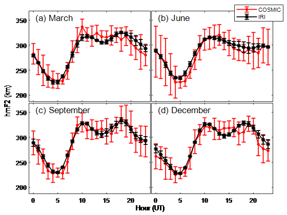
Corresponding comparisons between COSMIC-2 hmF2 measurements and IRI hmF2 values are illustrated in Figure 3. The figure shows that the electron densities peak at altitudes between 200 and 350 km, depending on the time of the day and season. In a pattern that is somewhat similar to the NmF2, the altitudes of peak electron density are higher during the day (after sunrise) and lower at night (after sunset). The troughs of the hmF2 diurnal profiles usually occur at around 04:00 to 05:00 UT, while the crests occur between 10:00 and 18:00 UT. Figure 3 also shows that there is good agreement between hmF2 values from both systems; the IRI model values are well within the error limits of the COSMIC-2 measurements and the patterns of both profiles are identical, showing that the IRI model does effectively reproduce the COSMIC-2 hmF2 measurements. The correlation coefficients between the COSMIC-2 and IRI hmF2 values (shown in Table 3) are consistently greater than 0.95 for all seasons. The RMSD values are typically ~ 10 km and less, translating to percentage RMSDs that are less than 4% for all four seasons. The results generally show that there is better agreement between the hmF2 values than between the NmF2 values.
Table 3: Table of correlation coefficients, RMSDs, and percentage RMSDs, computed between COSMIC-2 hmF2 measurements and IRI model values.
| Season | Correlation coefficient | RMSD (km) | Percentage RMSD (%) |
| March equinox | 0. 96 | 19.74 | 3.37 |
| June solstice | 0.98 | 7.79 | 2.79 |
| September equinox | 0.98 | 7.42 | 2.54 |
| December solstice | 0.96 | 10.33 | 3.61 |
4. Conclusion
First climatology of the NmF2 and hmF2 parameters using COSMIC-2 RO measurements in the equatorial African region is studied. There was the presentation of altitudinal electron density profiles from the COSMIC-2 mission, alongside corresponding ionosonde measurements and IRI model values. The results showed that the COSMIC-2 and ionosonde measurements were more closely related, while the IRI typically overestimated both measurements, especially at the F2 peak altitude and above. However, this study not only validates the use of COSMIC-2 data for ionospheric research in equatorial Africa but also brings attention to the need for model improvements and offers new perspectives on the vertical structure of the ionosphere in the region. These contributions are particularly valuable given the limited observational infrastructure available in West Africa equatorial and reinforce the potential of satellite-based measurements in supporting ionospheric monitoring and modeling efforts.
Diurnal profiles of the NmF2 and hmF2 were constructed from both COSMIC-2 and IRI on a seasonal basis using the medians of the values for each of the seasons, binned hourly.
The results generally showed a significant correlation (correlation coefficients greater than 0.9) between the COSMIC-2 and IRI model values. Typical differences between the COSMIC-2 and IRI NmF2 values were in the range of ~ 1.1 ×10⁵ to 1.7 ×10⁵ electrons/cm3, corresponding to percentage RMSDs of ~ 29% to 36%. The RMSDs were lower during the solstices and greater during the equinoxes, implying that the IRI model values were closer to the COSMIC-2 measurements during the solstices than during the equinoxes. This could be a result of the relatively lower electron densities recorded in the equatorial region during the solstices than during the equinoxes, and so the justification for computing the percentage RMSDs. The percentage RMSD was lowest for the March equinox season (~29%), and closely followed by values for the solstices (~30%). The greatest differences (both RMSD and percentage RMSD) were recorded during the September equinox (~35%). There was also an investigation of the differences between the COSMIC-2 measurements and the IRI values for three different phases of a diurnal profile (rising, peak, and decline phases). The results showed that the least differences (both RMSDs and percentage RMSDs) were usually obtained during the rising phase, while the greatest differences were usually obtained during the decline phase.
It was conspicuously observed that during the decline phase; the IRI model generally overestimated the COSMIC-2 NmF2 observations. The was a generally good agreement between the COSMIC-2 hmF2 measurements and the IRI model values, with RMSDs less than ~ 10 km and less, and percentage RMSDs less than 4%. Aside from the new results of electron density, NmF2, and hmF2 variations presented for the African equatorial African region using COSMIC-2 measurements, the paper also provides vital information on the climatologic differences between the IRI model predictions and the COSMIC-2 measurements, for improving ionospheric modeling in the region. However, the IRI model shows better in producing peak height (hmF2) than peak density (NmF2), this result will enhance understanding of model reliability across different ionospheric parameters.
Conflict of Interest
The authors declare no conflict of interest.
Acknowledgment
Radio occultation electron density data from the COSMIC-2 mission was used in this work. The authors are grateful to the sponsors and operators of the COSMIC-2 mission; the National Science Council and National Space Organization (NSPO), the National Oceanic and Atmospheric Administration (NOAA), the University Corporation for Atmospheric Research (UCAR), the National Science Foundation (NSF), National Aeronautics and Space Administration (NASA). Ionosonde electron density data was obtained from DIDBASE GIRO (https://ulcar.uml.edu/DIDBase/) through the SAO Explorer software. The authors are grateful to the GIRO team for providing and granting access to the ionosonde data. The authors acknowledge the OMNIWEB (https://omniweb.gsfc.nasa.gov/form/dx1.html) for providing and granting access to DST data used in this work. The first author is grateful to the University Support Program (USP) of the Centre for Atmospheric Research (CAR) for the support they provided using R&D funds from the Federal Government of Nigeria, and to the University of Nigeria – Nsukka (UNN) for approving the request to visit the Space Environment Research Facility of CAR.
- N.P. Chapagain, L. Patangate, “Ionosphere and its influence in communication systems,” An annual publication of Central Department of Physics, 10, 2016.
- V.L. Bychkov, G.V. Golubkov, A.I. Nikitin, The atmosphere and ionosphere, Springer, 2010.
- P.K. Bhattacharjee, “Fundamental to electromagnetic waves,” International Journal of Trend in Scientific Research and Development, 7, 454-462, 2023.
- R.K. Cole, E.T. Pierce, “Electrification in the earth’s atmosphere for altitudes between 0 and 100 kilometers,” Journal of Geophysical Research, 70(12), 2735-2749, 1965.
- R.A. Vincent, “The dynamics of the mesosphere and lower thermosphere: a brief review,” Progress in Earth and Planetary Science, 2, 1-13, 2015.
- M. Atiq, “Historical review of ionosphere in perspective of sources of ionization and radio waves propagation,” Research & Reviews: Journal of Space Science & Technology, 7(2), 28-39, 2018.
- O.A. Ogunmodimu, Auroral Radio Absorption: Modelling and Prediction, Ph.D Thesis, Lancaster University (United Kingdom), 2016.
- A. Daniel, G. Tilahun, A. Teshager, “Effect of ionosphere on radio wave propagation,” International Journal of Research, 3(9), 65-74, 2016.
- E.V. Appleton, “Wireless studies of the ionosphere,” Institution of Electrical Engineers- Proceedings of the Wireless Section, 7(21), 257-265, 1932.
- K.G. Budden, The propagation of radio waves: the theory of radio waves of low power in the ionosphere and magnetosphere, Cambridge University Press, 1988.
- H. Sizun, P. de-Fornel, Radio wave propagation for telecommunication applications, 35-67, Springer, Berlin, 2005.
- S. Dubey, R. Wahi, A.K. Gwal, “Ionospheric effects on GPS positioning,” Advances in Space Research, 38(11), 2478-2484, 2006.
- D. Atlas, R.C. Beal, R.A. Brown, D.P. Mey, R.K. Moore, C.G. Rapley, C.T. Swift, “Problems and future directions in remote sensing of the oceans and troposphere: a workshop report,” Journal of Geophysical Research: Oceans, 91(C2), 2525-2548, 1986.
- A.J. Mannucci, C.O. Ao, W. Williamson, “GNSS radio occultation,” Position, Navigation, and Timing Technologies in the 21st Century: Integrated Satellite Navigation, Sensor Systems, and Civil Applications, 1, 971-1013, 2020.
- R. Notarpietro, M. Cucca, S. Bonafoni, “GNSS signals: a powerful source for atmosphere and Earth’s surface monitoring,” Remote Sensing of Planet Earth, 171-200, 2012.
- S. Jin, R. Jin, X. Liu, GNSS atmospheric seismology, Springer, Berlin/Heidelberg, Germany, 2019.
- R. Padullés, E. Cardellach, K.N. Wang, C.O. Ao, F.J. Turk, M.D.L. Torre-Juárez, “Assessment of global navigation satellite system (GNSS) radio occultation refractivity under heavy precipitation,” Atmospheric Chemistry and Physics, 18(16), 11697-11708, 2018.
- Y.A. Liou, A.G. Pavelyev, J. Wickert, T. Schmidt, A.A. Pavelyev, “Analysis of atmospheric and ionospheric structures using the GPS/MET and CHAMP radio occultation database: a methodological review,” GPS Solutions, 9, 122-134, 2005.
- C.O. Ao, G.A. Hajj, T.K. Meehan, D. Dong, B.A. Iijima, A.J. Mannucci, E.R. Kursinski, “Rising and setting GPS occultations by use of open-loop tracking,” Journal of Geophysical Research, 114, D04101, 2009, doi:10.1029/2008JD010483.
- Y.H. Chu, C.L. Su, H.T. Ko, “A global survey of COSMIC ionospheric peak electron density and its height: a comparison with ground-based ionosonde measurements,” Advances in Space Research, 45, 431-439, 2010.
- M.M. Hoque, N. Jakowski, “A new global model for the ionospheric F2 peak height for radio wave propagation,” Annales Geophysicae, 30, 797–809, 2012.
- L. Hu, B. Ning, L. Liu, B. Zhao, Y. Chen, G. Li, “Comparison between ionospheric peak parameters retrieved from COSMIC measurement and ionosonde observation over Sanya,” Advances in Space Research, 54, 929-938, 2014.
- E.R. Kursinski, G.A. Hajj, J.T. Schofield, R.P. Linfield, K.R. Hardy, “Observing Earth’s atmosphere with radio occultation measurements using the Global Positioning System,” Journal of Geophysical Research: Atmospheres, 102(D19), 23429-23465, 1997.
- S. Mukherjee, S. Sarkar, P.K. Purohit, A.K. Gwal, “Seasonal variation of total electron content at crest of equatorial anomaly station during low solar activity conditions,” Advances in Space Research, 46(3), 291-295, 2010.
- D. Okoh, H. JohnBosco, R. Babatunde, S. Gopi, B.W. Joshua, O. Joseph, O. Olivier, M.M. Tshimangadzo, “Storm‐time modeling of the African regional ionospheric total electron content using artificial neural networks,” Space Weather, 18(9), e2020SW002525, 2020.
No related articles were found.