
Enhancing Long Time-Series Data Augmentation with Generative Adversarial Networks

Adv. Sci. Technol. Eng. Syst. J. 11(3), 40–48 (2026);
 DOI: 10.25046/aj110303
With the development of deep learning, time-series-related tasks have been increasingly applied across various fields. However, time-series data used in the medical and semiconductor industries are often different from those in daily life, with high sampling frequencies and very long sequence lengths, and collecting such data is usually very challenging. Therefore, data augmentation is a significant part of applying such long time-series data to deep learning tasks.
In this study, the autoregressive model used in the TimeGAN method is replaced with IndRNN to generate long time-series data. The experimental results also show that, as the sequence length increases, this simple substitution can achieve a strong data augmentation effect and gradually extend to longer time-series data. Furthermore, the practical use of the generated time-series data in stock prediction tasks demonstrates the effectiveness of data augmentation, particularly for longer time-series data. This practical application provides a more direct illustration of the capability to perform data augmentation for long time-series data.
1. Introduction
Time-series data is a common type of information in our daily lives, encompassing data that varies over time, such as weather observations, stock prices, traffic flow, sensor records, and medical records. This data type is ubiquitous across many domains, including time-series prediction, anomaly detection, and classification. For instance, using past weather time-series data can help meteorologists predict future weather trends. In the financial sector, stock price prediction is of significant importance to investors and traders. Similarly, in traffic management, leveraging time-series data on traffic flow can optimize routes and traffic control.
In these tasks, having sufficient data is crucial to avoid overfit-ting in learning models. However, collecting certain time-series data can be challenging, particularly in manufacturing, semiconductor, and medical fields. For example, in the manufacturing and semiconductor industries, data may be difficult to obtain due to confidentiality concerns or because the processes that generate it are costly. Additionally, privacy concerns related to patient information make acquiring large-scale medical data challenging. Furthermore, these time-series data differ from general weather or stock data as they often have very high sampling frequencies and can be extremely long, spanning hundreds of thousands of time steps. These reasons underscore the significance of data augmentation for long time-series data to effectively increase training data diversity and improve model generalization.
Inspired by relevant tasks, our objective is to perform data aug-mentation on sensor data from silicon wafer processing machines with high sampling frequencies and sequence lengths approaching 200,000. To achieve this, we employ the Time-series Generative Adversarial Network (TimeGAN), a generative adversarial network (GAN) based method for generating time-series data. TimeGAN uses an autoencoder architecture to map real data into a latent space and then reconstruct it. Adversarial training in the latent space enhances TimeGAN’s ability to capture complex structures and temporal dependencies in time-series data.
To generate even longer time-series data, we replace the autoregressive model in TimeGAN, originally based on GRU, with IndRNN. Compared to traditional RNNs such as GRU and LSTM, IndRNN has the advantage of independent weights, making it more effective at handling long time-series data. Traditional RNNs can suffer from vanishing or exploding gradients due to the cumulative effect of recurrent weights, which limits network depth and length. However, the independent weights of IndRNN mitigate these issues and enable efficient training on longer time-series data.
The generated data is compared with real data using visualiza-tion, discriminative scores, and predictive scores. These metrics enable observation of whether the generated data shows a similar distribution to the real data and whether it captures the temporal dependencies and structures present in the real data. The experi-mental results demonstrate that TimeGAN with IndRNN performs on par with the original TimeGAN using GRU and even surpasses it for long time series. This paper is an extension of work originally presented in conference IS3C 2025 [1].
In summary, the contributions of this study are as follows:
- The autoregressive model employed in TimeGAN was re-placed with IndRNN, allowing the model to generate long time-series data and effectively augment long time-series
- Despite the limitations on sequence length handling by In-dRNN,the experiments show that this straightforward sub-stitution successfully increases the sequence length of time-series data generated by TimeGAN.
2. Related Works
2.1. Long Time-series Data
The concept of ”long time series” varies across studies: some treat them as model inputs, while others treat them as forecastting outputs. For input modeling, Dual-Path RNN (DPRNN) [2] segments sequences into overlapping chunks, using intra- and inter-chunk RNNs to capture local and global dependencies. This approach achieves strong speech separation performance with reduced model size.
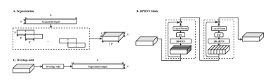
To address the limitations of traditional RNNs on long sequences, LSSL [3] integrates RNNs, convolutions, and neural differential equations in a linear state-space framework, though it is computationally intensive. S4 [4] improves on this by decomposing the state matrix and applying frequency-domain computation, resulting in better performance and efficiency.
For long sequence prediction, Informer extends the Transformer architecture with Probsparse self-attention, attention distillation, and a generative-style decoder, significantly improving forecasting accuracy and efficiency. These developments illustrate ongoing progress in modeling long-term time series from both input and output perspectives across various applications.
2.2. Time-series Data Augmentation based on GAN
Generative Adversarial Networks (GANs) [5] have been widely used for data augmentation in image, audio, and time-series modeling areas. GANs can generate realistic synthetic samples by learning data distributions, thereby enhancing model generalization, especially when real data is scarce. However, time-series data presents unique challenges, including temporal dependencies, multivariate structures, and high dimensionality.
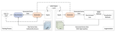
Based on LSTM, TS-GAN [10] incorporates techniques such as the Wasserstein loss, 1D convolution, and a sequential squeeze-and-excitation (SSE) module to enhance generation quality. It has shown strong results on health-related datasets, outperforming earlier methods.
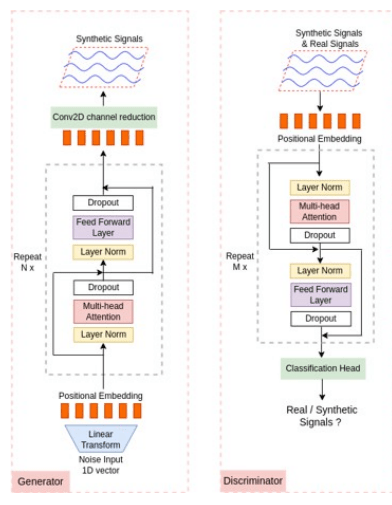
Early models, such as C-RNN-GAN [6] and RCGAN [7], applied recurrent structures to sequential data in biosignal and real-world time series applications. To address the limitations of RNN based GANs, TSS-GAN [8] introduced a Transformer-based architecture [9] that treats time series as image-like inputs and uses patch-based self-attention to model irregular dependencies and variable-length sequences.
These advances demonstrate how architectural and training improvements have significantly enhanced the effectiveness of GAN-based time-series data augmentation.
3. Method
3.1. Overview
This study is a Time-series Generative Adversarial Network (TimeGAN)[11] architecture based on an Independently Recur-rent Neural Network (IndRNN) [12]. The model aims to generate long time-series data, and its architecture is illustrated in Figure 4. TimeGAN utilizes an autoencoding component to learn the representation of time-series data in the latent space and an adversarial component for adversarial learning to generate synthetic time-series data that resembles the original data. The architecture of the model is illustrated in Figure 5.
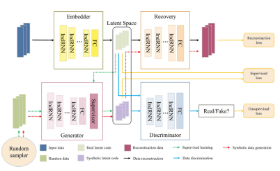
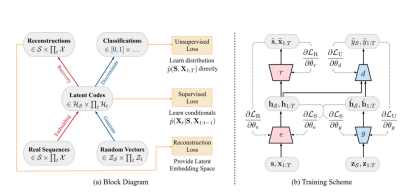
To address TimeGAN’s limitation in generating long time-series data, the autoregressive model used in its components, originally based on GRU, is replaced with IndRNN. By doing so, the goal of generating long time-series data is pursued. The generation process of TimeGAN for time-series data is shown in Figure 4 as the red solid line. It starts with a random sampler that generates random vectors, followed by the generator, which generates synthetic latent codes in the latent space. Finally, the recovery component converts the synthetic latent codes back into time-series data, represented as the reconstruction data in Figure 4.
3.2. Independently Recurrent Neural Network (IndRNN)
As shown in Figure 4, this study uses IndRNN to construct all core components of TimeGAN, including the embedder, recovery, generator, and discriminator. Traditional RNNs follow the recurrence formula:
\[
\mathbf{h}_{t}
=
\sigma
\left(
\mathbf{W}\mathbf{x}_{t}
+
\mathbf{U}\mathbf{h}_{t-1}
+
\mathbf{b}
\right)
\tag{1}
\]
However, they suffer from vanishing or exploding gradients due to repeated matrix multiplications. While LSTM and GRU mitigate this with gating mechanisms, they still rely on saturating activation, which limits deep training.
IndRNN addresses this by assigning independent recurrent weights to each neuron. The hidden state update for the n-th neuron is defined as:
\[
h_{n,t}
=
\sigma
\left(
w_n x_t
+
u_n h_{n,t-1}
+
b_n
\right)
\tag{2}
\]
This design decouples neurons and allows direct control of gradient flow, enabling stable training over long sequences. Thus, IndRNN is better suited for long-time series generation.
3.3. The Backpropagation Through Time for an IndRNN
Because neurons in each layer are independent, gradient back-propagation in IndRNN can be computed independently across layers. Assuming the objective Jn at time T , the gradient concerning the hidden state hn,t:
\[
\frac{\partial J_n}{\partial h_{n,t}}
=
\frac{\partial J_n}{\partial h_{n,T}}
\frac{\partial h_{n,T}}{\partial h_{n,t}}
=
\frac{\partial J_n}{\partial h_{n,T}}
\prod_{k=t}^{T-1}
\frac{\partial h_{n,k+1}}{\partial h_{n,k}}
\]
\[
=
\frac{\partial J_n}{\partial h_{n,T}}
\prod_{k=t}^{T-1}
\sigma’_{n,k+1} u_n
=
\frac{\partial J_n}{\partial h_{n,T}}
u_n^{T-t}
\prod_{k=t}^{T-1}
\sigma’_{n,k+1}
\tag{3}
\]
This design decouples neurons and allows direct control of gradient flow, enabling stable training over long sequences. Thus, IndRNN is better suited for long-time series generation.
Here, σ′ is the derivative of the activation function, and un is the neuron-specific recurrent weight. Since activation derivatives are typically within 0 and 1, the gradient magnitude is primarily controlled by un a trainable parameter.
This formulation enables direct control of gradient flow via un, allowing IndRNN to mitigate vanishing and exploding gradients and achieve stable training over long sequences.
3.4. Time-series Generative Adversarial Networks
In 2019, Yoon proposed TimeGAN, a time-series generative model that integrates autoencoding and adversarial learning. It consists of an embedder, a recovery module, a generator, and a discriminator. The autoencoder maps data to a latent space and re-constructs it, while the GAN components generate synthetic latent codes and distinguish them from real ones. Joint training enables the generator to produce realistic sequences as the discriminator improves until synthetic data becomes indistinguishable from real data.
3.5. The Objective of TimeGAN
Let = X = {(xn,1:T )}N be a multivariate time-series dataset with Nn n=1 and T , and each time samples, where each sequence has length n step xn,t ∈ H, the feature space. These sequences follow a joint distribution p(S, X1:T ), and the objective is to learn an approximate distribution pˆ(S, X1:T ) that closely matches the true distribution.
3.6. Training Autoencoding Component
The autoencoding part consists of an embedder and a recovery component. Its main purpose is to facilitate the conversion between features and latent codes in the latent space, allowing the adversarial part to learn in a lower-dimensional space.
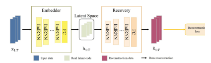
The embedder takes the input data features and transforms them into a latent-space representation (latent codes). The embedder can be represented by the following equation:
\[
\mathbf{h}_t
=
e\left(
\mathbf{h}_{t-1},
\mathbf{x}_t
\right)
\tag{4}
\]
where xt is the feature of input data, e represents the embedder, and ht represents the latent codes, which is the expression in the latent space. Next, the recovery component takes the latent codes zlatent and reconstructs them back into the original time-series features. The recovery process can be represented by the following equation:
\[
\tilde{\mathbf{x}}_{t}
=
r\left(
\mathbf{h}_{t}
\right)
\tag{5}
\]
where r is the recovery, the recovered time-series features are denoted as x˜t. To learn the relationship between these recovered features and the latent codes, the reconstruction loss LR is utilized to compare the original features x1 : T with the reconstructed features x˜1 : T . The objective is to make the reconstructed features as close as possible to the original ones. The reconstruction loss LR is defined as follows:
\[
\mathcal{L}_{R}
=
\mathbb{E}_{\mathbf{x}_{1:T}\sim P}
\left[
\sum_{t}
\left\|
\mathbf{x}_{t}
–
\tilde{\mathbf{x}}_{t}
\right\|_{2}
\right]
\tag{6}
\]
3.7. Training Only with Supervised Loss
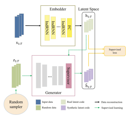
In TimeGAN, the generator takes a random input sequence z1:T and produces synthetic latent codes. The generation process is defined as:
\[
\hat{\mathbf{h}}_{t}
=
g\left(
\hat{\mathbf{h}}_{t-1},
\mathbf{z}_{t}
\right)
\tag{7}
\]
To guide learning, a supervised loss encourages the generated codes hˆ1:T to resemble real latent codes h1:T from the embedder.
During training, the generator uses ht−1 (from real data) rather than its own outputs to better capture the true temporal dynamics.
The supervised loss LS is defined as:
\[
\mathcal{L}_{S}
=
\mathbb{E}_{\mathbf{x}_{1:T}\sim P}
\left[
\sum_{t}
\left\|
\mathbf{h}_{t}
–
g\left(
\mathbf{h}_{t-1},
\mathbf{z}_{t}
\right)
\right\|_{2}
\right]
\tag{8}
\]
This loss aligns synthetic and real latent sequences, enabling the generator model to capture realistic temporal dependencies more effectively.
3.8. Training Adversarial Component
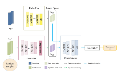
The final component of TimeGAN is the adversarial module, consisting of a generator and a discriminator that operate in the latent space. The generator produces synthetic latent codes hˆ1:T , and the discriminator aims to distinguish them from real latent codes h1:T .
Given input h˜, the discriminator output at the time is:
\[
\tilde{\mathbf{y}}_{t}
=
d\left(
\tilde{\mathbf{u}}_{t}
\right),
\qquad
\tilde{\mathbf{u}}_{t}
=
\tilde{\mathbf{c}}_{t}
\left(
\tilde{\mathbf{h}}_{t},
\tilde{\mathbf{u}}_{t-1}
\right)
\tag{9}
\]
The unsupervised adversarial loss is defined as:
\[
\mathcal{L}_{U}
=
\mathbb{E}_{\mathbf{x}_{1:T}\sim P}
\left[
\sum_{t}
\log y_{t}
\right]
+
\mathbb{E}_{\hat{\mathbf{x}}_{1:T}\sim \hat{P}}
\left[
\sum_{t}
\log\left(1-\hat{y}_{t}\right)
\right]
\tag{10}
\]
The discriminator maximizes LU to distinguish real from fake sequences. At the same time, the generator minimizes it to produce sequences indistinguishable from real data. This adversarial process helps the generator learn realistic temporal dynamics and align the synthetic distribution with the original.
3.9. Optimization
Let θe, θr, θg and θd represent the parameters of the embedder, recovery, generator, and discriminator, respectively. The autoencoding components are trained by minimizing:
\[
\min_{\theta_e,\theta_r}
\left(
\lambda \mathcal{L}_{S}
+
\mathcal{L}_{R}
\right)
\tag{11}
\]
where λ ≥ 0 balances the supervised loss LS and the reconstruction loss LR, encouraging accurate feature reconstruction and latent alignment.
For the adversarial components, the optimization is defined as:
\[
\min_{\theta_g}
\left(
\eta \mathcal{L}_{S}
+
\max_{\theta_d}\mathcal{L}_{U}
\right)
\tag{12}
\]
where η ≥ 0 weights the supervised loss and LU is the unsupervised adversarial loss. This setup promotes realistic generation in the latent space, balancing the generator’s realism with the discriminator’s ability to distinguish real and fake sequences.
4. Implementation
4.1. Data Preprocess
Before training, timestamp fields are removed, as explicit time is not used. The long time series is segmented into overlapping sub-sequences of fixed length using a sliding window. The resulting data has shape [n, seqlen, instances], where n is the number of sub-sequences. Min-max normalization is applied to scale values to [0, 1], followed by random shuffling to approximate an i.i.d. dataset for training.
4.2. Data Postprocess
After generation, inverse min-max scaling restores the syn-thetic data to its original value range. Due to prior shuffling, the generated sub-sequences remain i.i.d. and cannot be reconstructed into a single long sequence—this aligns with standard practices in time-series data generation, ensuring the synthetic data follows the original distribution.
5. Experimental Results
5.1. Datasets
Stocks. This dataset contains Google’s daily stock prices from 2004 to 2019, including opening, highest, lowest, closing, adjusted closing prices, and trading volume. The data in this dataset represent continuous time series, and the features are correlated.
Traffic. The UCI Metro Interstate Traffic Volume dataset [13] includes temperature, rainfall, snowfall, cloud cover, weather cate-gory, and traffic flow for each hour. The features in this dataset are not correlated.
Table 1: The information of the datasets
| Dataset | Seq. length | Instances | Avg. len | Sampling rate |
|---|---|---|---|---|
| Stock | 3,773 | 6 | 24 days | 1 day |
| Traffic | 48,204 | 6 | 24 hrs | 1 hr |
5.2. Experimental Settings
Sequence length. The chosen datasets have an average length of 24, and the experimental setup involves progressively increasing the sequence length. Specifically, the experiments are conducted using sequence lengths of 24, 72, 144, 288. This approach enables a comprehensive assessment of the proposed data augmentation method across varying time scales.
Batch size. To address longer training times in some experi-ments, the batch size was increased during training. Three different batch sizes were considered: 128, 256, and 512.
Hidden dimension. In the experiments, the hidden dimension was set to 4 times the number of instances in the dataset, following the TimeGAN reference. This choice was made because, in certain cases where the original data dimension is relatively small, a higher hidden dimension can help generate time-series data that closely resembles the real data.
5.3. Evaluation Metrics
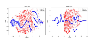
Visualization. To compare the distributions of original and generated data, two dimensionality reduction techniques, PCA [14] and t-SNE [15], are employed to project high-dimensional data into two-dimensional space. A greater overlap between the two distributions indicates higher similarity between the generated and real data. PCA captures the global variance of the data, while t-SNE preserves local structures and neighborhood relationships, providing complementary perspectives on distributional similarity. In the visualization plots, red points denote the original data and blue points denote the generated data, allowing an intuitive view of how closely the two distributions align.
Discriminative score. In this evaluation, original data are la-beled as “real” and generated data as “fake.” A time-series classifier is trained to distinguish between the two. If the classifier fails to differentiate them, the generated data are considered highly simi-lar to the original data. The ideal case occurs when the classifier achieves an accuracy of 0.5, indicating indistinguishability. The discriminative score is defined as;
\[
\mathrm{discriminative\_score}
=
\left|
\mathrm{discriminator\_accuracy}
–
0.5
\right|
\tag{13}
\]
A lower discriminative score indicates greater similarity be-tween generated and original data. As the score approaches zero, the generated data more closely resembles the original data, reflecting effective data augmentation.
Predictive score. The generated data should preserve the char-acteristics of the original data by capturing its evolving conditional distribution over time. To evaluate this, a predictor is trained to forecast the next time step for each input sequence, using generated data for training and original data for testing. The Mean Absolute Error (MAE) is adopted as the evaluation metric, with lower predic-tive scores indicating greater similarity between the generated and original data in terms of temporal dependencies and distributional dynamics.
Three training–testing settings are considered to assess augmen-tation effectiveness: “Train on real, test on real” (TRTR) serves as the baseline; “Train on mix (real + synthetic), test on real” (TMTR) provides the most representative measure of augmentation benefit by leveraging both datasets during training; and “Train on synthetic, test on real” (TSTR) represents the most challenging scenario, as insufficient quality in generated data may degrade performance on real data. These settings enable a comprehensive evaluation of the proposed data augmentation approach.
5.4. Result on Stock Dataset
In the experimental results on the Stock dataset, although our proposed method performs slightly worse than TimeGAN, the differences in the discriminative and predictive scores are within 0.01. At a sequence length of 288, our approach yielded a discriminative score lower than TimeGAN’s. However, the predictive score across different data combinations remained slightly higher than that of TimeGAN.
Table 2: Discriminative score & Predictive score on Stock Dataset
| Sequence length | Discriminative score ↓ | Predictive score ↓ | |||||
|---|---|---|---|---|---|---|---|
| TimeGAN | Ours | TRTR | TSTR | TMTR | |||
| TimeGAN | Ours | TimeGAN | Ours | ||||
| 24 | 0.0561 | 0.125 | 0.038 | 0.0402 | 0.0468 | 0.0378 | 0.0439 |
| 72 | 0.1362 | 0.138 | 0.0361 | 0.0366 | 0.042 | 0.0360 | 0.0368 |
| 144 | 0.0986 | 0.1059 | 0.035 | 0.0402 | 0.0435 | 0.0357 | 0.0408 |
| 288 | 0.1381 | 0.1232 | 0.0327 | 0.0379 | 0.0382 | 0.0338 | 0.0366 |
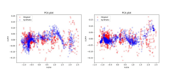
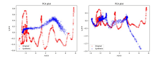
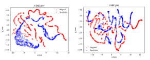
However, solely relying on discriminative scores and predictive scores may not directly indicate the intuitive quality of the gener-ated data. Hence, we use two-dimensional visualization plots to assess whether the distribution of generated data resembles that of the original data. In all the following two-dimensional visualization plots, red dots represent the original data, while blue dots represent the generated data. The more the distributions overlap, the more similar the generated data is to the original data.At a sequence length of 24, both TimeGAN and our proposed method achieve good results, though some areas are sparsely covered in the visualization plots.
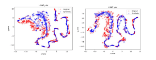
At sequence length = 72, as the sequence length increases, learning the distribution of the original data becomes more challenging for both our proposed method and TimeGAN. There are some differences between the results of the two methods, with our method paying less attention to sparsely populated regions and focusing on secondary, densely populated areas for learning.
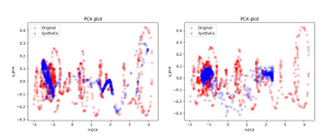
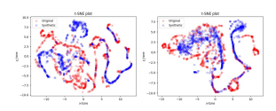
At sequence length = 144, the challenge of learning the distribution of the original data becomes even more evident. In the PCA visualization plots, TimeGAN covers only a very small portion of the original data and has a completely different distribution. In contrast, our proposed method not only covers more densely populated regions of the original data but also captures its distribution in the middle, even if it does not overlap directly.
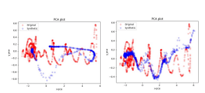
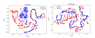
At last, at sequence length = 288, the difficulty in learning increases further as the sequence length grows. For a sequence length of 144, both methods yield subpar results, but our proposed method shows minimal overlap with the original data in both PCA and t-SNE visualization plots. Moreover, the trend of the generated data is more similar to that of the original data in our proposed method than in TimeGAN.
5.5. Results on Traflc Dataset
The experimental results on the Traffic dataset in Table 3 reveal that both the proposed method and TimeGAN perform poorly on the discriminative, predictive, and visualization scores. One reason for this unsatisfactory performance is the dataset’s characteristics. Unlike the Stock dataset, the Traffic dataset lacks inter-instance correlations, making it more challenging for models to learn from the data. Moreover, the Traffic dataset has a significantly longer total sequence length compared to the stock dataset. While IndRNN, the chosen model for our method, can handle sequences up to 5,000, learning sequences with a total length of over 40,000 becomes exceptionally challenging. In conclusion, the lack of inter-instance correlation and the substantial increase in total sequence length in the Traffic dataset make learning difficult, resulting in unsatisfactory performance for both the proposed method and TimeGAN.
Table 3: Discriminative score & Predictive score on Traffic Dataset
| Sequence length | Discriminative score ↓ | Predictive score ↓ | ||
|---|---|---|---|---|
| TimeGAN | Ours | TimeGAN | Ours | |
| 24 | 0.3488 | 0.4547 | 0.2266 | 0.2484 |
| 72 | 0.4763 | 0.4864 | 0.2682 | 0.2306 |
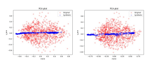
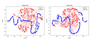
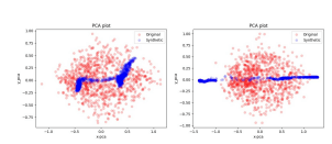
Figure 19: PCA visualization on Traffic Dataset with sequence length = 72. On the left, the TimeGAN method is utilized, and on the right, our proposed method is applied.
5.6. Stock Forecasting
To further validate the effectiveness of this augmentation approach, the generated data was practically applied to stock pre-diction tasks. The subsequences of the generated data are independently identically distributed. Consequently, with a generated data sequence length of 24, all feature values from time steps t − 23, t − 22, …, t − 1 were utilized to forecast the trading volume at time step t. In this experiment, a simple 3-layer LSTM model was employed as the prediction model, trained for 250 epochs. Similar to the prediction score discussed in previous section, various combinations were used for training and testing. However, as the aim was to assess this data augmentation approach, only the TRTR and TMTR data combinations were utilized. The Mean Absolute Error (MAE) was adopted as the evaluation metric, with lower scores indicating better performance.
Table 4: The result of stock forecasting
| Sequence length | MAE loss ↓ | ||
|---|---|---|---|
| TRTR | TMTR | ||
| TimeGAN | Ours | ||
| 24 | 0.0274 | 0.0285 | 0.0263 |
| 72 | 0.0259 | 0.0263 | 0.0281 |
| 144 | 0.0266 | 0.0264 | 0.0265 |
| 288 | 0.0274 | 0.0268 | 0.0268 |
6. Conclusion
The four main components of TimeGAN, including the embedder, recovery, generator, and discriminator, were replaced with IndRNN. The objective was to perform data augmentation on long time-series data through this simple substitution. By gradually increasing the time-series length in experiments on a stock dataset, it was observed that data augmentation achieved satisfactory results as the time-series length increased. This indicates efficacy in augmenting long time-series, demonstrating potential for extension towards even longer time-series. Furthermore, applying the generated data to stock prediction tasks also yielded superior results on longer time series than models using solely original data. This practical application further supports the notion that the approach is beneficial for augmenting long time-series data. While IndRNN can handle relatively long time series, it may not be feasible for practical applications involving ultra high sampling frequencies and sequence lengths exceeding hundreds of thousands. The maximum time-series length that IndRNN can handle is approximately five thousand. Therefore, for future real-world applications, alternative approaches such as Dual-path RNN [2] or S4 [4] could be explored to handle such extremely long time-series data. The experimental results in Table 4 reveal that although our approach yielded slightly higher scores than TimeGAN for sequence lengths of 72 and 144, for longer sequence lengths such as 144 and 288, the proposed method consistently outperformed TRTR. This observation indicates the efficacy of this augmentation method for longer time series.
- L.-C. Lin, M.-C. Yu, C.-K. Chiang, “Long Time-series Data Augmentation via Timeseries Generative Adversarial Network,” in International Symposium on Computer, Consumer and Control (IS3C), 2025, doi:10.1109/IS3C65361.2025.11131006.
- Y. Luo, Z. Chen, T. Yoshioka, “Dual-path rnn: efficient long sequence modeling for time-domain single-channel speech separation,” in ICASSP 2020-2020 IEEE International Conference on Acoustics, Speech and Signal Processing (ICASSP), 46–50, IEEE, 2020, doi:10.1109/ICASSP40776.2020.9054266.
- A. Gu, I. Johnson, K. Goel, K. Saab, T. Dao, A. Rudra, C. Ré, “Combining recurrent, convolutional, and continuous-time models with linear state space layers,” Advances in neural information processing systems, 34, 572–585, 2021, doi:10.5555/3540261.3540305.
- A. Gu, K. Goel, C. Re, “Efficiently Modeling Long Sequences with Structured State Spaces,” in International Conference on Learning Representations, 2022.
- I. Goodfellow, J. Pouget-Abadie, M. Mirza, B. Xu, D. Warde-Farley, S. Ozair, A. Courville, Y. Bengio, “Generative adversarial nets,” Advances in neural information processing systems, 27, 2014, doi:10.5555/2969033.2969125.
- O. Mogren, “C-RNN-GAN: Continuous recurrent neural networks with adversarial training,” arXiv preprint arXiv:1611.09904, 2016, doi:10.48550/arXiv.1611.09904.
- C. Esteban, S. L. Hyland, G. Rätsch, “Real-valued (medical) time series generation with recurrent conditional gans,” arXiv preprint arXiv:1706.02633, 2017, doi:10.48550/arXiv.1706.02633.
- X. Li, V. Metsis, H. Wang, A. H. H. Ngu, “Tts-gan: A transformer-based time-series generative adversarial network,” in International Conference on Artificial Intelligence in Medicine, 133–143, Springer, 2022, doi:10.1007/978-3-031-09342-5_13.
- A. Vaswani, N. Shazeer, N. Parmar, J. Uszkoreit, L. Jones, A. N. Gomez, Ł. Kaiser, I. Polosukhin, “Attention is all you need,” Advances in neural information processing systems, 30, 2017, doi:10.5555/3295222.3295349.
- Z. Yang, Y. Li, G. Zhou, “TS-GAN: Time-series GAN for Sensor-based Health Data Augmentation,” ACM Transactions on Computing for Healthcare, 4(2), 1–21, 2023, doi:10.1145/3583593.
- J. Yoon, D. Jarrett, M. Van der Schaar, “Time-series generative adversarial networks,” Advances in neural information processing systems, 32, 2019, doi:10.5555/3454287.3454781.
- S. Li, W. Li, C. Cook, C. Zhu, Y. Gao, “Independently recurrent neural network (indrnn): Building a longer and deeper rnn,” in Proceedings of the IEEE conference on computer vision and pattern recognition, 5457–5466, 2018, doi:10.1109/CVPR.2018.00572.
- J. Hogue, “Metro Interstate Traffic Volume,” UCI Machine Learning Repository, 2019, doi:10.24432/C5X60B.
- F. B. Bryant, P. R. Yarnold, “Principal-components analysis and exploratory and confirmatory factor analysis,” 1995.
- L. Van der Maaten, G. Hinton, “Visualizing data using t-SNE,” Journal of machine learning research, 9(11), 2008, doi:10.5555/1756006.1953016.