1. Introduction

The credit card debt crisis has been a major concern in the capital market and among card-issuing institutions for many years. Credit cards and cash-card debts are abused by most card users, regardless of their payment capabilities. This crisis poses a great threat to both cardholders and banks. The payment default means the failure to pay the credit card bills. Researchers have attempted to forecast the credit card customers’ default payments using machine learning techniques [1]. The public’s lack of understanding of basic financial principles, as seen by the recent financial crisis, has proven that they are unable to make sound financial judgments.

Individuals’ minimum monthly credit card payments should be researched in depth to discover the link between consumer income, payment history, and future default payments [2]. Increasing consumer finance confidence, to avoid delinquency is a big challenge for cardholders and banks as well. In a well-established financial system, risk assessment is more important than crisis management [2]. With historical financial data, for example, business financial statements, client transaction and reimbursement records, etc., we can predict business execution or individual clients’ default risk and lessen the harm and instability. To make accurate customer risk assessments for their credit services department, banks are required by having sophisticated credit scoring systems to automate the credit risk scoring tasks [3]. Management of the credit risk for the banking sector and financial organizations have extensively started to gain importance. Developing an automated system to accurately forecast the probability of cardholder’s future default, will help not only to manage the efficiency of consumer finance but also effectively handle the credit risk issues encountered in the banking sector [3], [4].

Individual firms have been gathering massive amounts of data every day in the era of big data. Finding the relevant information from data and turning that information into meaningful outcomes is a big issue for businesses. As a result, in this article, we investigate the risk of failure to pay the minimum credit card amount, which is a transaction that should be done monthly. The Generalized Linear Model (GLM), single classification tree, and random forest are compared to predict the credit default risk. Prediction accuracy and interpretability are the two main factors we consider when selecting the final model. The principal component analysis (PCA) is used to reduce the data dimensionality.

2. Literature Review

Machine learning is the act of automatically or semi-automatically exploring and analyzing massive amounts of data to uncover significant patterns and rules [5]. It has been utilized in different types of financial analysis such as predicting money laundering, stock analysis, detection of bankruptcy, the decision of loan approval, etc. [6, 7]. Machine learning algorithms are inadequately used for detecting default payments of credit card users. Different kinds of research are ongoing to improve the accuracy of machine learning algorithms in predicting default payment of credit card users, and a small portion of improvement plays a vital role in the economic developments of the related organizations [8, 9]. Before the 1980s, some statistical methods such as Linear Discriminant Analysis (LDA) [10], and Logistic Regression (LR) [11] were used to estimate the credit default probability. Starting from the 1990s, machine learning methods such as K-nearest neighbor (KNN) [12], neural network (NN) [13], genetic algorithm [14], and support vector machine (SVM) [15] were used to assess the default risk of credit card users. In 2018, researchers compared 5 data mining methods on credit card default prediction: logistic regression, SVM, neural network, Xgboost, and LightGBM [16]. In 2020, AdaBoost was employed to build credit default prediction models [17]. In 2020, researchers investigated the credit card default prediction in the imbalanced data sets [18].

However, the GLM is rarely used in credit card default prediction. GLM has the advantage of easy interpretability and implementation. We believe it’s worthwhile to apply the GLM in the research of credit card payment default prediction. In this paper, we will compare the GLM with the decision tree and random forest and explain its advantages.

3. Data Description and Exploratory Analysis

3.1.  Data description

The data set came from the credit cardholders from a major bank in Taiwan in October 2005, with a total of 25000 records. The target variable to be predicted in this data is a binary variable – default payment (Yes = 1, No = 0). Table 1 lists the 25 variables in the data including all the predictors and the target variable (default status). The first 5 of the predictors are demographic characteristics. The next 6 variables are about the status of past payments. The further 6 variables are about the amount of the past bill statement. The next 6 variables are about the amount of paid bills and the last 2 predictors are the limit balance of individuals and the default status of the client. This credit payment data has a typical characterization of imbalanced datasets in terms of the target variable, for 5529 records (22.12%) are the records of default and 19471 records (77.88%) are non-default payments.

Table 1: Data dictionary

VARIABLE NAME	DESCRIPTION	FACTOR LEVELS
ID	The ID of each client	Values
SEX	Gender	1=male 2=female
EDUCATION	The level of education of each client	·         0= Unknown ·         1=graduate school ·         2=university ·         3=high school ·         4=others
MARRIAGE	Marital Status	1=married 2=single, 3=others
AGE	Age in years	Ages
LIMIT_BAL	The amount of given credit in NT dollars includes individual and family credit	Numerical NT Dollars
·         PAY_0	Repayment status in September 2005	·         -2=payment made two months earlier, -1=pay duly, 0=paid right before due ·         1=payment delay for one month, 2=payment delay for two months, … 8=payment delay for eight months,)
PAY_2	Repayment status in August 2005	scale same as above
PAY_3	Repayment status in July 2005	scale same as above
PAY_4	Repayment status in June 2005	scale same as above
PAY_5	Repayment status in May 2005	scale same as above
PAY_6	Repayment status in April 2005	scale same as above
·         BILL_AMT1:	amount of bill statement in September 2005	Numerical NT dollars
BILL_AMT2:	Amount of bill statement in August 2005	Numerical NT dollars
BILL_AMT3	Amount of bill statement in July 2005	Numerical NT dollars
BILL_AMT4	Amount of bill statement in June 2005	Numerical NT dollars
BILL_AMT5	Amount of bill statement in May 2005	Numerical NT dollars
BILL_AMT6	Amount of bill statement in April 2005	Numerical NT dollars
PAY_AMT1	Amount of previous payment in September 2005	Numerical NT dollars
PAY_AMT2	Amount of previous payment in August 2005	Numerical NT dollars
PAY_AMT3	Amount of previous payment in July 2005	Numerical NT dollars
PAY_AMT4	Amount of previous payment in June 2005	Numerical NT dollars
PAY_AMT5	Amount of previous payment in May 2005	Numerical NT dollars
PAY_AMT6	Amount of previous payment in April 2005	Numerical NT dollars
default.payment.next.month	Default Status	1=Yes 0=No

3.2.  Explore the relationship between the predictors and the target variable

In this section, relations between the predictors vs the target variable will be explored using graphs.

Figure 1 is the stacked histogram that shows the distribution of the credit limit (limit balance) among defaulting records (blue bars) and non-defaulting records (pink bars).

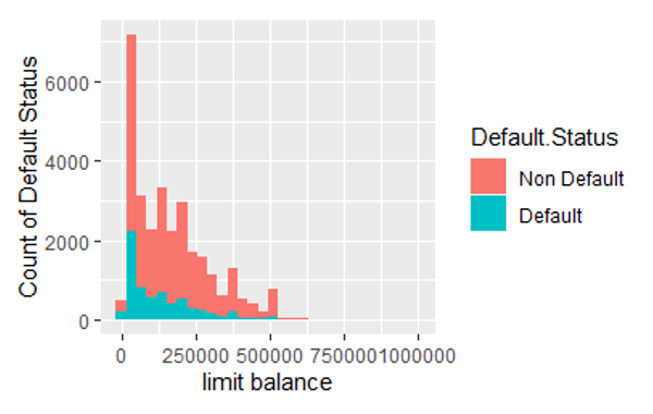
Figure 1: The stacked histogram of the credit limit in default records and non-default records.

From Figure 1, we can observe the default records have a higher proportion of Lower LIMIT_BAL values than non-defaulting records. To confirm this observation, we did a two-sample t-test with a null hypothesis mean of LIMIT_BAL in the non-default group is less than in the default group. The p-value is less than 10e-15 which means we can confidently accept the alternative hypothesis: the mean of LIMIT_BAL in the non-default group is higher than in the default group. This confirms our observation in Figure 1. This conclusion matches the reality that lower credit balances are usually issued to credit users with higher default risk. This distinctive characteristic of the predictor LIMIT_BAL indicates it’s a good variable to predict default.

Table 2: Some details of hypothesis tests.

Alternative Hypothesis	Type of Hypothesis Test	P-value
The mean of LIMIT_BAL in the non-default group is greater than in the default group	T-test	<2.2
The chance of default at age 25-40 is lower than at other ages.	Two-proportions z-test	<2.2

Figure 2 shows the distribution of the age among default credit users and non-default users, using a density histogram. We observe the non-default group has a higher proportion of age 25-40, but a lower proportion of other ages. This makes us infer the age 25-40 has a lower chance of default. To confirm this as the alternative hypothesis, we did a two-proportions z-test. The P-value as shown in Table 2 is very significant and confirms our hypothesis. The reason age 25-40 has a lower default rate could be people in this age range are in the working-age, healthy, and don’t have much financial burden from their family yet. In contrast, people younger than 25 may have not started their careers yet, therefore with little to no income. People older than 40 could be less healthy, retired, or need financial support from their families such as children’s college education. The above discussion indicates the variable Age can be a good predictor.

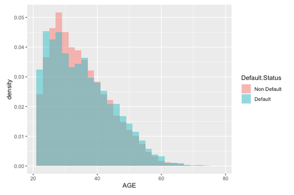
Figure 2: The stacked histogram of age in default records and non-default records.

Figure 3 represents the default status distribution within different gender. The percentage of defaults in males (24%) is slightly higher than in females (20%). To confirm this difference is statistically significant, we did a two-proportion z-test with the alternative hypothesis that male has a higher default chance than female. The p-value of this z-test is 2.47 , which means we should accept the alternative hypothesis. This confirms our observation. This difference is probably because females are more conservative when managing their personal finance than males, which results in lower default risk. This difference indicates the variable Sex is a good predictor.

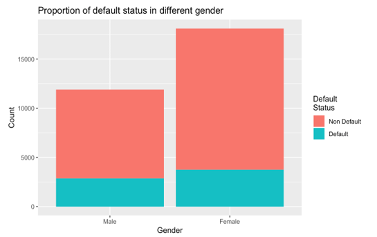
Figure 3: Distribution of default and non-default records in males and females.

Figure 4 displays the proportion of education levels in non-default and default records. It shows that the non-default records have a larger proportion of higher educated individuals from graduate school and university levels. This also matches our intuition that higher education levels associate with higher income and lower default risk. To statistically confirm this observation, we did a two-proportion z-test with an alternative hypothesis that non-default users have a higher proportion of education level of university or graduate school. The p-value of this test is 0.00226, which confirms our observation.

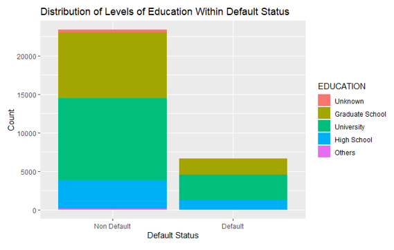
Figure 4: The distribution of education level in default and non-default.

Figure 5 displays the proportion of different lateness in the last statement payment (PAY_0) in default records and non-default records. The variable PAY_0 has more proportion of “On Time” or “Early” values in the non-default records than in default values. We also did a two-proportions z-test to confirm this observation as the alternative hypothesis in the z-test. The p-value of the test is less than 2.2 , which confirms the alternative hypothesis. This means that being current or ahead of payments is associated with non-defaulting in the following month. Therefore the lateness in the last statement payment (PAY_0) is a good predictor to predict the default. For the lateness of the last 2nd payment to the last 7th payment (PAY_1 to PAY_6), we observed the same pattern. That is, non-default records have a higher proportion of “On Time” or “Early” payments in each of the past 7 months than default records. This suggests the payment statuses in the past months have potentially strong predictive power on the default risk.

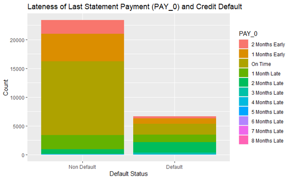
Figure 5: The distribution of PAY_0 values in non-default and default values. Variable PAY_0 is the lateness of the last statement payment

3.3.  Reduce the levels of factor variables to increase the predictive power

If a factor variable in the data has too many different values (levels), its predictive power is usually lower. This is because the factor variable is often expanded as the combination of multiple dummy variables when predicting the target variable, where each dummy column is one possible value of the factor variable. If there are many possible values in the variable, then this expanded data will have too many columns versus the number of rows. The data rows will not be long enough compared with its dimensionality to train a highly accurate and robust algorithm. To reduce the data dimensionality, we need to reduce the levels of the factor variables by combining similar levels, so the prediction accuracy can be improved.

Table 3 shows the number of non-default and default records in the factor variable Education. According to this table, the university and high school education have higher proportions of defaults than the other values. We combine these 2 levels as one level and name it “HighSchoolUniversity”. Since “others” and “unknown” have a lower proportion of default, they will be combined and named ‘others’. The factors are then reduced to HighSchoolUniversity, Graduate School, and Others.

Table 3: Data dictionary

EDUCATION	Non-default	Default	Total	Proportion of default
Unknown	319	26	345	8%
Graduate School	8549	2036	10585	19%
University	10700	3330	14030	24%
High School	3680	1237	4917	25%
Others	116	7	123	6%

Table 4: The proportion of non-default in each level of predictor PAY-0 before its levels combined.

PAY _0	Non Default	Default	Total	Proportion of default
2 Months Early	2394	365	2759	13%
1 Month Early	4732	954	5686	17%
On Time	12849	1888	14737	13%
1 Month Late	2436	1252	3688	34%
2 Months Late	823	1844	2667	69%
3 Months Late	78	244	322	76%
4 Months Late	24	52	76	68%
5 Months Late	13	13	26	50%
6 Months Late	5	6	11	55%
7 Months Late	2	7	9	78%
8 Months Late	8	11	19	58%

Table 4 shows the number of non-default and default records in the factor variable PAY_0. The values of non-default in PAY_0 = “2 Months Early”, “1 Month Early”, and “On Time” have a similar lower proportion of defaults than the other PAY_0 values. We combine these 3 levels as one level and name it “Pay duly”. Also, the PAY_0 = “2 Months Late” or more have a similarly high proportion of default and it will be reasonable to combine them as one level. PAY_0 = “1 Month Late” stands as the other level. Therefore the number of levels in predictor PAY_0 is reduced to 3.

3.4.  Using Kernel Principal Component Analysis to generate a new feature

The predictors in this data may not be independent of each other. The predictors SEX, EDUCATION, and MARRIAGE might be related to each other. For instance, the male may have higher education, but a lower percentage of getting married compared with female. We can use the kernel principal component analysis (Kernel-PCA) [19] to generate new variable(s) to represent the related variables so that the dimensionality of the data can be further reduced. The kernel-PCA works better than PCA when nonlinear relation exists between initial variables in the data. Since there is an interaction between the variables according to our later discussion in session 4.2, such nonlinear relation exists. We run the kernel-PCA on the data that only contains the three variables SEX, EDUCATION, and MARRIAGE to find out the principle components among them. Table 5 is the kernel-PCA results showing the first 4 principal components (PC). The first 4 principal components combined can describe 87% of the variation.

Table 5: The importance of the first 2 principal components.

	PC1	PC2	PC3	PC4
Proportion of variance	0.270	0.240	0.207	0.153
Cumulative Proportion	0.270	0.511	0.718	0.871

The new features PC1, …, PC4 will replace the total 8 levels in the variables SEX, EDUCATION, and MARRIAGE in the later predictive modeling to predict the target variable.

4. Methodology

In this session, we will introduce the main idea of GLM and apply it to the data pre-processed in previous sessions. The decision tree and random forest algorithms will also be applied to compare the GLM. The data was split into training (70%) and test (30%) set for each of the algorithms.

4.1.  Introduction of GLM

The ordinary linear regression assumes the target variable follows the normal distribution. However, the target variables in many real-world data don’t follow the normal distribution. For instance, personal income follows a lognormal distribution with the majority of people in middle income and few are super-rich. In the credit data used in this paper, the target variable is a binary variable that obviously doesn’t follow the normal distribution. For the non-normal distributed target variable, the ordinary linear regression no longer works. The GLM is the generalized version of the linear regression that works for a broader range of target variables including non-normal and normal distributed. The GLM uses a link function to transform the non-normal target variable to normal distributed, then the ordinary regression method can be used.

4.2.  Select an Interaction

Even though the generalized linear model (GLM) is a linear model, it can still deal with the non-linear relation. That’s done by including the interaction term. The interaction means the relationship between one predictor and the target changes when the value of another predictor changes. This suggests the two predictors are not independent of each other but exist in interaction between them.

In Figure 6, we look at how education and marriage interact. Individuals who are married and are in high school have a larger proportion of non-default than those who are single. However, individuals who are single and are in higher education have a higher proportion of non-default than married people. This might be because single people spend less than married people and have a higher proportion of non-default. It is also worth noting that there are more singles in higher education than married people who are in higher education, as well as a large number of married high school graduates. We observe that at each level of education the number of people who are married and will default varies with no pattern hence we will select this interaction between marriage and education.

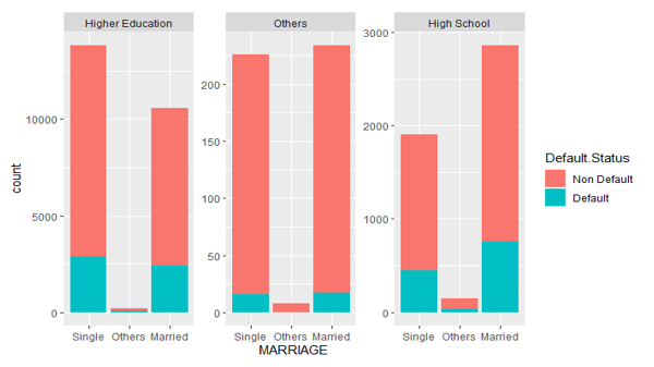
Figure 6: The distribution of default status with Education for each marital level.

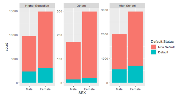
Figure 7: The distribution of default status with Education for each gender.

The interaction between education and sex is explored in Figure 7. There are much more females in all three levels of education who will default than males. Females, on average, have a greater degree of education than males and are less likely to default. There is an interaction between sex and education because of the pattern it has in each educational level.

We do the same thing to explore the interaction between MARRIAGE and SEX using Figure 8. When SEX = “male”, the married male has a significantly lower default risk than the single males. However, when SEX = “female”, the default risk is not significantly different between the single females and married females. To explain this, we can regard it’s often the men who pay more bills in the marriage. Married men should take more financial responsibility after getting married than single men. Therefore they have higher default risk. While for females, such financial responsibility in marriage is not so significant, thus there is not much difference in terms of default risk between married females and single females. Therefore, the SEX value impacts.

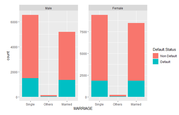
Figure 8: The distribution of default status with Gender for Marital status

4.3.  Link Function Selection

We need to specify the distribution of the target variable and what link function to be used. Our target variable is binary, which is either “default” or “not default”, the natural choice of the target distribution is binomial.

For the link function, it must map the prediction to the zero to one range because we will first predict the probability of default, then classify it. The binomial distributed GLM has four candidates for the link functions: logit, probit, Cauchit, and cloglog. They will all map the regression result to a value between 0 and 1, which can be regarded as the payment default probability. Table 6 provided details about these 4 link functions.

In Table 6, the  is the regression equation.  is the target variable. With the link function, the target variable is transformed into a normal distributed variable that can be regressed using the regular least squares method. The AIC is used as an important metric when we decide which link function to choose. Each link function is tried on the training data and the AIC of its GLM is listed in the last column of Table 6. The Cauchit link and Cloglog link have higher AIC, so we exclude them. The Logit and Probit have similar small AIC, so either of them can be chosen as the link function. Since the Logit link is the canonical link for binary family and it’s more widely used, we decide to choose Logit function as the link function.

Table 6: Four link functions for binary distribution and its AIC on our training data.

Name	Link Function	Response Probability	AIC on training data
Logit			18388
Probit			18386
Cauchit			18451
Cloglog			18468

4.4.  Feature selection

Feature selection (also known as variable selection, attribute selection, or variable subset selection) is the technique of selecting a subset of relevant features (predictors and variables) for use in the development of a model. It is the automatic selection of the most significant and relevant qualities contained in the data for predictive modeling [20]. Forward selection and backward selection are the two main types of feature selection methods. Forward selection is an iterative approach in which the model starts with no variables. This method keeps adding up the variable that improves the model the most (measured by AIC) in each iteration until adding a new variable no longer enhances the model’s performance. The AIC of forward selection is 18380. The backward selection begins with all the variables (full model) and removes the least significant variable one after the other until its AIC no longer decreases. The AIC of backward selection is 18390.  The best model solely depends on the defined evaluation criterion of which the AIC was used. Since forward selection has a lower AIC, it’s used as the feature selection method. This choice removed variables Age, PC2, PC3, PC4, BILL_AMT3,4,5, PAY_AMT3,5  by not selecting them. The area under curve (AUC) for the test data is reduced to 0.7637 with an AIC decreasing to 18442.

4.5.  Data Sampling and G-K-Fold Cross-validation.

To ensure the distribution is unchanged after data is spitted into the training set and testing set, we use stratified sampling. Both sets contain the same portion of credit default data after the data partition. To analyze the accuracy and stability of different algorithms, the G-K-fold stratified cross-validation is used. In K-fold stratified cross-validation, the data is stratified partitioned into K equal parts, where each part of the data has the same distribution for the target variable. 1 part of this data is defined as the testing data, the remaining K-1 parts of the data are the training data. G-K-folder stratified cross-validation will do the K-folder stratified cross-validation for G times, to generate enough results for algorithms performance evaluation statistically.

4.6.  Interpretation of the GLM Results

Table 7 listed the results of the regression coefficients of the GLM. It’s the trained GLM model generated from the training data using the features we selected from the step-AIC method based on the new features built from kernel-PCA and variables interaction considered. The “Estimate” column contains the regression coefficients. According to this table, the following variables, levels or interactions are significantly important in predicting the default payment, due to the small p-value and relatively large estimated coefficients:

• PAY_0 = 1 month late
• PAY_0 = More than a month late
• PAY_2 = More than a month late
• PAY_3 = More than a month late
• PAY_4 = More than a month late
• PAY_5 = More than a month late
• PAY_6 = More than a month late
• EDUCATIONOthers:MARRIAGESingle

This makes sense. The PAY_0 is more important than the other payment status variables because it’s the most recent payment status. The PAY_0=More_than_a_month_late has a larger estimated coefficient than PAY_0=1_month_late because the former level is associated with a higher probability of default payment, and both levels result in a higher chance of default compared with PAY_0 paid in time. The negative coefficients of interaction levels between EDUCATION and MARRIAGE mean they indicate a lower probability of default payment.

Table 7: Summary of the GLM results.

	Estimate			Std. Error		z value		Pr(>|z|)		Signif. Codes
(Intercept)	-10.51			22.62		-0.47		0.64
BILL_AMT1	<1E-4			<1E-4		-2.69		0.01		**
BILL_AMT2	<1E-4			<1E-4		3.78		<1E-3		***
BILL_AMT6	<1E-4			<1E-4		-3.10		<1E-2		**
PAY_AMT1	<1E-4			<1E-4		-5.32		<1E-4		***
PAY_AMT2	<1E-4			<1E-4		-2.55		0.01		*
PAY_AMT4	<1E-4			<1E-4		-0.82		0.41
Limit.Balance	<1E-4			<1E-4		-6.86		<1E-4		***
PAY_AMT6	<1E-4			<1E-4		-2.93		0.00		**
PAY_01 month late	0.78			0.06		13.10		< 2E-16		***
PAY_0More than a month late	2.00			0.06		30.92		< 2E-16		***
PAY_21 month late	-1.26			1.05		-1.20		0.23
PAY_2More than a month late	0.23			0.07		3.17		<1E-3		**
PAY_31 month late	-10.33			228.91		-0.05		0.96
PAY_3More than a month late	0.27			0.07		3.79		<1E-4		***
PAY_41 month late	0.87			397.31		0.00		1.00
PAY_4More than a month late	0.21			0.08		2.76		0.01		**
PAY_5More than a month late	0.27			0.08		3.20		<1E-3		**
PAY_6More than a month late	0.33			0.07		4.49		<1E-4		***
PC1	0.72			2.04		0.35		0.72
PC2	-2.57			2.57		-1.00		0.32
PC3	-2.66			4.09		-0.65		0.52
PC4	-4.28			4.00		-1.07		0.28
EDUCATIONHigher Education:MARRIAGESingle	11.16			22.68		0.49		0.62
EDUCATIONOthers:MARRIAGESingle	-51.98			35.15		-1.48		0.14
EDUCATIONHigh School:MARRIAGESingle	-4.97			13.57		-0.37		0.71
EDUCATIONHigher Education:MARRIAGEOthers	-45.27			55.01		-0.82		0.41
EDUCATIONOthers:MARRIAGEOthers	-88.72			127.20		-0.70		0.49
EDUCATIONHigh School:MARRIAGEOthers	-53.17			38.30		-1.39		0.17
EDUCATIONHigher Education:MARRIAGEMarried	16.43			34.10		0.48		0.63
EDUCATIONOthers:MARRIAGEMarried	-48.24			41.72		-1.16		0.25
EDUCATIONHigh School:MARRIAGEMarried	NA			NA		NA		NA
—
Signif. codes:  0 ‘***’ 0.001 ‘**’ 0.01 ‘*’ 0.05 ‘.’ 0.1 ‘ ’ 1

The trade-off between sensitivity (or TPR) and specificity (1 –FPR) is depicted by the ROC curve. Classifiers with curves that are closer to the top-left corner perform better. A random classifier is supposed to offer diagonal points (FPR = TPR) as a baseline. The test becomes less accurate as the curve approaches the 45-degree diagonal of the ROC space to the left. The area beneath the ROC curve is referred to as the AUC [21]. To generate the ROC curve, we use the roc() function in R’s pROC library by comparing the model prediction probability vs the real target value. The ROC curve of this GLM method on the test data is provided in figure 9 and it has an AUC of 0.757.

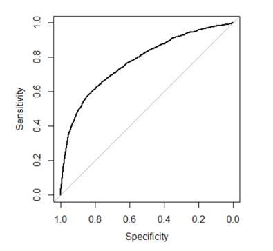
Figure 9: ROC curve of the GLM model

4.7.  Classification Tree

Classification tree methods (i.e., decision tree methods) are recommended when the machine learning task contains classifications or predictions of the outcome. A Classification tree labels, records, and assigns variables to discrete classes. A Classification tree is built through a process known as binary recursive partitioning. This is an iterative process of splitting the data into partitions and then splitting it up further on each of the branches. Before constructing a tree, the data was split into training (70%) and testing (30%) sets.

We use the rpart package in R to implement the decision tree. With its tree structure, the decision tree can automatically incorporate the non-linear relation between variables. Therefore, we don’t need to add the interaction term (SexEduMarriage) as the input variable. All the variables in the original data are included as the input variables to build the decision tree. Gini impurity is used to split the tree. Figure 10 is the classification tree produced.

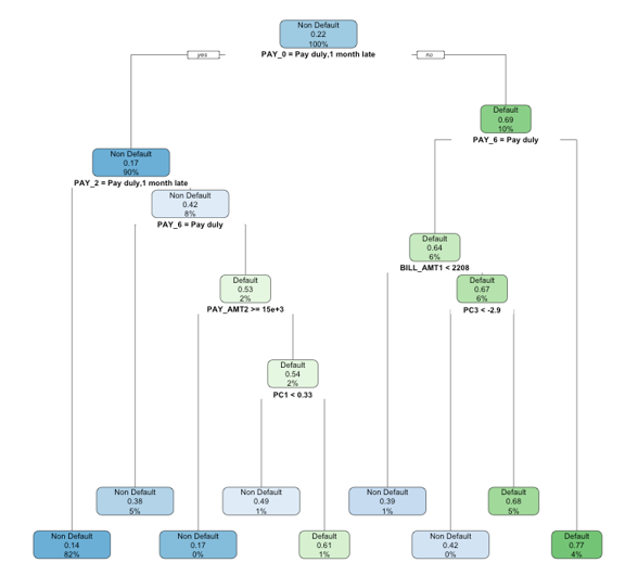
Figure 10: Classification tree result.

A confusion matrix is used to check the performance of a classification model on a set of test data for which the true values are known. Most performance measures such as precision, and recall are calculated from the confusion matrix. We can observe in Table 8 that the confusion matrix of our test data has the true positive to be 6633 with a small false positive of 1253 and there is a false negative of 376 and a true negative of 737, with a classification accuracy of 0.8188.

Table 8: Confusion Matrix of decision tree on the test data

		Reference
		Non Default	Default
Prediction	Non Default	6633	1253
	Default	376	737

The classification tree in figure 10 indicates that the variable PAY_0 is the most important variable to predict the default risk because it’s the variable used to split the first node in the tree. This classification tree algorithm has an accuracy rate of 0.819 and AUC of 0.6966 which is lower than the GLM. Figure 11 provides the ROC curve of this algorithm.

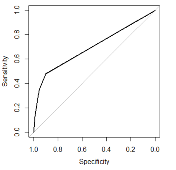
Figure 11: ROC curve for classification tree

4.8.  Random Forest

Random forest, as its name implies, consists of many individual decision trees that operate as an ensemble. Each tree in the random forest splits out a class prediction and the class with the most votes becomes our model’s final prediction. The random forest can also return the importance of each predictor as shown in Table 9. The results are scaled, so the numbers indicate relative importance. Generally, variables that are used to make the split more frequently and earlier in the trees in the random forest are determined to be more important. According to Table 9, Pay_0 is the most important variable to predict the default payment. This matches the GLM results in Table 7, where the coefficients of the two levels of Pay_0 are highly significant and have large values. The new variable SexEduMarriage that was created by us has an importance of 2.263, which means it was not used frequently in any of the trees. This agrees with the single tree built previously, where the variable SexEduMarriage is not used in any of the split nodes.

Table 9: The relative importance of each predictor variable

	Relative Importance
AGE	392.04
PAY_0	651.78
PAY_2	238.91
PAY_3	189.40
PAY_4	116.50
PAY_5	115.35
PAY_6	77.57
BILL_AMT1	424.41
BILL_AMT2	391.97
BILL_AMT3	376.45
BILL_AMT4	354.90
BILL_AMT5	353.91
BILL_AMT6	356.20
PAY_AMT1	378.61
PAY_AMT2	343.74
PAY_AMT3	330.01
PAY_AMT4	318.30
PAY_AMT5	313.88
PAY_AMT6	328.04
Limit.Balance	371.19
PC1	139.72
PC2	132.30
PC3	149.37
PC4	142.92

The ROC curve of this random forest algorithm is given in figure 12. Its AUC is 0.7639.

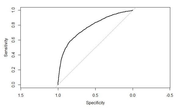
Figure 12: ROC curve for Random Forest

5. Results Comparison and Conclusion

As we mentioned in session 4.5, the G-K-fold stratified cross-validation is used to collect the AUCs and other metrics of each algorithm. We set G=10, K=10. That is in total 100 runs for each algorithm based on different training and testing data partitions. To compare the 3 algorithms, we consider the mean of AUCs, accuracy, sensitivity, specificity, positive predictive value (PPV), negative predictive value (NPV), run time with the corresponding standard deviation, and 95% confidence interval for each classifier. They are listed in Table 10.1-10.3. The metrics of GLM are significantly better than the decision tree and comparable to the random forest.

All 3 algorithms are implemented in R and run on a MacBook Pro 2018 with 2.2 GHz 6-Core Intel Core i7, 16 GB 2400 MHz DDR4 memory, and macOS Catalina. We found the GLM runs 7.7 times faster than the decision tree, and 45.7 times faster than the random forest. This is also a big advantage of GLM versus the other 2 algorithms. The details of run time are also listed in tables 10.1-10.3.

Table 10.1: Mean of metrics for 3 algorithms

	Mean
	GLM	Decision Tree	Random Forest
AUC	0.764	0.693	0.762
Accuracy	0.820	0.820	0.817
Sensitivity	0.357	0.350	0.361
Specificity	0.952	0.954	0.946
PPV	0.678	0.683	0.656
NPV	0.839	0.838	0.839
Run time	0.108	0.830	4.931

Table 10.2: Standard deviation of metrics for 3 algorithms

	Standard Deviation
	GLM	Decision Tree	Random Forest
AUC	0.0051	0.0047	0.0057
Accuracy	0.0027	0.0027	0.0028
Sensitivity	0.0092	0.0191	0.0104
Specificity	0.0022	0.0052	0.0029
PPV	0.0116	0.0165	0.0123
NPV	0.0020	0.0034	0.0021
Run time	0.0245	0.0649	0.2310

Table 10.3: Standard deviation of metrics for 3 algorithms

	95% Confidence Interval
	GLM	Decision Tree	Random Forest
AUC	[0.756, 0.776]	[0.685, 0.703]	[0.75, 0.77]
Accuracy	[0.814, 0.826]	[0.815, 0.826]	[0.812, 0.822]
Sensitivity	[0.342, 0.376]	[0.312, 0.381]	[0.343, 0.38]
Specificity	[0.948, 0.956]	[0.944, 0.963]	[0.941, 0.952]
PPV	[0.655, 0.7]	[0.65, 0.716]	[0.637, 0.678]
NPV	[0.836, 0.843]	[0.832, 0.844]	[0.836, 0.843]
Run time	[0.088, 0.136]	[0.734, 0.977]	[4.658, 5.682]

DeLong test is used to compare the GLM, decision tree, and random forest classifiers AUCs. We did the DeLong test for GLM vs decision tree with alternative hypnosis “GLM has higher AUCs than decision tree”, another DeLong test for GLM vs random forest with alternative hypnosis “GLM has lower AUCs than random forest”. The ROC curves for each pair of algorithms obtained in each run of the G-K-fold crossed validation are used as the input for the DeLong test. Therefore, for each pair of algorithms, G K DeLong test is computed. The p-values of these tests are recorded, and their mean, standard deviation are reported in Table 11. The p-value of the DeLong test of GLM vs decision tree is extremely small, so we should accept its alternative hypothesis that GLM has higher AUCs than the decision tree. For the GLM vs random forest DeLong test, its p-value is 0.8628, so we should accept its null hypothesis that GLM has higher AUCs than random forest. A boxplot is given in Figure 13 to summarize the comparison of AUCs obtained from the cross-validation for all 3 algorithms. Both DeLong tests and the boxplot show the superiority of GLM vs the other 2 algorithms.

Table 11: DeLong test to compare AUCs.

	GLM vs Decision Tree	GLM vs Random Forest
Alternative hypothesis	GLM has higher AUCs than the decision tree	GLM has lower AUCs than random forest
Mean of p-value	4.71E-38	0.6617
SD of p-value	4.70E-37	0.2530

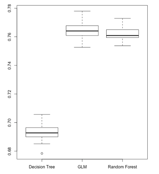
Figure 13: Boxplot to summarize the AUCs comparison.

To discuss the stability of different classifiers, we use the coefficient of variation (CV) of AUC. The CV is defined as the standard deviation divided by the mean. A better classifier is the one with a smaller standard deviation of AUCs and higher average AUCs. The smaller CV of AUC means the algorithm is more stably accurate. We collected the AUCs for 3 algorithms from the G-K-fold cross-validation and calculate the CV of each algorithm’s AUCs. The result is listed in Table 12. It shows the 3 algorithms have the similar CV of AUCs.

Table 12: Coefficient of variation (CV) of AUCs.

	GLM	Decision Tree	Random Forest
CV of AUCs	0.00671	0.00676	0.00749

To summarize, the average AUCs for the single decision tree was 0.693 on the test data set, whereas the GLM had 0.764 and the random forest had 0.762. We don’t recommend the single decision tree as the final model because of its low AUC. For the remaining two algorithms, the GLM has several advantages over the random forest, one of which is its ease of implementation. The GLM regression formula can be clearly written using an algebra expression. The probability of a default payment can be easily calculated even with simple tools like a calculator or spreadsheet. However, for the random forest, it requires computer programming to obtain the results. Also, the GLM is easier to comprehend and interpret than the random forest, making it easier for credit card companies to grasp and make further business or management decisions upon it. One disadvantage of a GLM over the random forest is that it does not automatically incorporate variable interactions. In GLM, we need first to explore which variables could interact with each other and then manually add those interactions into the regression. The random forest can achieve this automatically. However, the random forest is prone to overfitting, especially when a tree is particularly deep. A small change in the data value could lead to totally different results if using the tree algorithms. Furthermore, the GLM uses fewer features than random forest because of the stepAIC forward selection applied for GLM. Last but not least, the GLM runs much faster than the random forest. Table 13 summarizes the comparison. Based on the above reasons, we conclude GLM model is a better model to predict the credit card default than the decision tree and random forest.

Table 13: Comparison of GLM with other two algorithms on credit card default prediction.

	GLM	Decision Tree	Random Forest
Average AUC	0.764	0.693	0.762
Interpretability	High	Medium	Low
Implementation	Easiest	Easy	Difficult
Overfitting risk	Low	Medium	High
Algorithm speed	Fast	Slower	Slowest

Conflict of Interest

The author declares no conflict of interest.

Acknowledgment

The author would like to thank the reviews for their valuable time spent on reviewing this paper, and for helpful suggestions to improve this paper.

1. M. Chou, “Cash and credit card crisis in Taiwan.” Business weekly: 24-27, 2006.
2. A. Subasi, S. Cankurt, “Prediction of default payment of credit card clients using Data Mining Techniques,” In 2019 International Engineering Conference (IEC), 115-120, IEEE, 2019, doi: 10.1109/IEC47844.2019.8950597.
3. A. Verikas, Z. Kalsyte, M. Bacauskiene, A. Gelzinis, “Hybrid and ensemble-based soft computing techniques in bankruptcy prediction: a survey,” Soft Computing, 14(9), 995-1010, 2010, doi: https://doi.org/10.1007/s00500-009-0490-5.
4. F.N. Koutanaei, H. Sajedi, M. Khanbabaei, “A hybrid data mining model of feature selection algorithms and ensemble learning classifiers for credit scoring,” Journal of Retailing and Consumer Services, 27, 11-23, 2015, doi: https://doi.org/10.1016/j.jretconser.2015.07.003.
5. M. Berry, G. Linoff, Mastering data mining: The art and science of customer relationship management. New York: John Wiley & Sons, Inc, 2000.
6. P. Giudici, “Bayesian data mining, with application to benchmarking and credit scoring,” Applied Stochastic Models in Business and Industry, 17(1), 69-81, 2001, doi:,https://doi.org/10.1002/asmb.425.
7. L. C. Thomas, “A survey of credit and behavioral scoring: Forecasting financial risk of lending to consumers,” International Journal of Forecasting, 16, 149–172, 2000, doi: https://doi.org/10.1016/S0169-2070(00)00034-0.
8. J. N. Crook, D. B. Edelman, L. C. Thomas, “Recent developments in consumer credit risk assessment,” European Journal of Operational Research, 183(3), 1447– 1465, 2007, doi: https://doi.org/10.1016/j.ejor.2006.09.100.
9. G. Derelioğlu, F. G. Gürgen, “Knowledge discovery using neural approach for SME’s credit risk analysis problem in turkey,” Expert Systems with Applications, 38(8), 9313– 9318, 2011, doi: https://doi.org/10.1016/j.eswa.2011.01.012.
10. E. I. Altman, “Financial ratios, discriminant analysis and the prediction of corporate bankruptcy,” The journal of finance, 23(4), 589–609, 1968, doi: https://doi.org/10.2307/2978933.
11. C. Verma, V. Stoffová, Z. Illés, S. Dahiya, “Binary logistic regression classifying the gender of student towards computer learning in European schools,” In The 11th Conference Of Phd Students In Computer Science (p. 45), 2018.
12. W. Henley, D. J. Hand, “A K‐Nearest‐Neighbour Classifier for Assessing Consumer Credit Risk,” Journal of the Royal Statistical Society: Series D (The Statistician), 45(1), 77-95, 1996, doi: https://doi.org/10.2307/2348414.
13. D. West, “Neural network credit scoring models,” Computers & Operations Research, 27(11), 1131–1152, 2000, doi: https://doi.org/10.1016/S0305-0548(99)00149-5.
14. S. Oreski, G. Oreski, “Genetic algorithm-based heuristic for feature selection in credit risk assessment,” Expert systems with applications, 41(4), 2052-2064, 2014, doi: https://doi.org/10.1016/j.eswa.2013.09.004.
15. T. Harris, “Credit scoring using the clustered support vector machine,” Expert Systems with Applications, 42(2), 741–750, 2015, doi: https://doi.org/10.1016/j.eswa.2014.08.029.
16. S. Yang, H. Zhang, “Comparison of several data mining methods in credit card default prediction,” Intelligent Information Management, 10(5), 115-122, 2018, doi: 10.4236/iim.2018.105010.
17. Y. Yu, “The application of machine learning algorithms in credit card default prediction,” In 2020 International Conference on Computing and Data Science (CDS), 212-218, IEEE, 2020, doi: 10.1109/CDS49703.2020.00050.
18. T. M. Alam, K. Shaukat, I. A. Hameed, S. Luo, M. U. Sarwar, S. Shabbir, J. Li, M. Khushi, “An investigation of credit card default prediction in the imbalanced datasets,” IEEE Access, 8, 201173-201198, 2020, doi: 10.1109/ACCESS.2020.3033784.
19. H. Hoffmann, “Kernel PCA for novelty detection,” Pattern recognition, 40(3), 863-874, 2007, doi: https://doi.org/10.1016/j.patcog.2006.07.009.
20. V. Kumar, S. Minz. “Feature selection: a literature review,” SmartCR, 4(3), 211-229, 2014, doi: 10.6029/smartcr.2014.03.007.
21. J. Huang, C. X. Ling, “Using AUC and accuracy in evaluating learning algorithms,” IEEE Transactions on knowledge and Data Engineering, 17(3), 299-310, 2005, doi: 10.1109/TKDE.2005.50.

(Click Here)