
Many-objective Placement Optimization in Virtual Network Functions
 , Fernando Ariel Britez Cantero, Luis Guillermo Moré Rodríguez*, Diego Pedro Pinto-Roa, Domingo Colbes Sanabria
Adv. Sci. Technol. Eng. Syst. J. 11(3), 9–39 (2026);
 DOI: 10.25046/aj110302
Network Functions Virtualization (NFV) poses the VNF placement problem under multiple, potentially conflicting objectives, such as Quality of Service (QoS), costs, and resource efficiency.
This work treats VNF placement as a many-objective optimization problem (MaOP) and presents two primary contributions: (i) a correlation analysis of state-of-the-art objectives to reduce dimensionality while maintaining representativeness, resulting in the selection of 11 key objective functions — specifically, energy cost, bandwidth consumption, latency, traffic load, resource fragmentation, maximum link utilization, licensing costs, SLO costs, distance traveled, number of VNF instances, and effective throughput; and (ii) a systematic comparison of many-objective evolutionary algorithms (R-VEA, NSGA-III, and MOEA/D) across multiple topologies (ZIB54, INDIA, and EON) under various load levels. Results demonstrate through non-parametric Friedman and Wilcoxon statistical testing (adjusted 𝑝 < 0.05 via Holm-Bonferroni) that R-VEA achieves superior overall performance. Its Angle-Penalized Distance (APD) metric effectively balances convergence and diversity across most scenarios, producing a Vargha-Delaney effect size (𝐴12) greater than 0.86 in most topologies compared to NSGA-III and MOEA/D. Conversely, MOEA/D exhibits competitive performance only in specific high-traffic edge cases (e.g., ZIB54 under extreme load), where it outpaces R-VEA due to front distortion. Taken together, the findings indicate that while no single algorithm dominates in every outlier condition, R VEA emerges as the most statistically consistent and robust solution for the 11-objective MaOP VNF placement problem. This contributes to ensuring QoS and reducing CAPEX/OPEX through high performance solutions along the Pareto front.
1. Introduction
Driven by the rapid growth of telecommunications in recent years, there is a critical need of network architectures that offer greater flexibility and lower costs while eliminating dependency on proprietary hardware vendors. Consequently, several studies propose decoupling network functions from hardware [1], refer-ring to traditional implementations as Physical Network Functions (PNFs) or hardware middleboxes. These consist of dedicated physical appliances designed to perform specific network tasks, such as transforming, inspecting, filtering or otherwise manipulating network traffic. Through these operations, various network objectives are achieved without compromising the Quality of Service (QoS) [2]. Common examples of such functions include firewalls, Deep Packet Inspection (DPI), Network Address Translation (NAT), WAN Optimization Controllers, Proxies, and Load Balancers [3] among others. Members of the European Telecommunications Standards Institute (ETSI) proposed virtualization to enable greater versatility in network functions, addressing the previously described challenges [4]. This gave origin to the term Network Function Virtualization (NFV). The main idea behind this is to build a network architecture that transforms the way to build and operate networks taking advantage of the standard IT virtualization technologies to consolidate network functions based on proprietary hardware of commercial devices [4].
Fundamentally, this technology entails replacing expensive dedicated hardware by software middleboxes, which are referred to as Virtual Network Functions (VNFs) in NFV terminology [5]. The adoption of this emergent technology results in significant reductions in Capital Expenditure (CapEx) and Operating Expenditure (OpEx), while simultaneously enhancing Quality of Service (QoS) for final users.
Several critical challenges exist within the NFV paradigm, most notably the Virtual Network Function Placement (VNF-P) problem, which is a central issue characterized by a NP-Hard complexity [6]. Various research efforts have addressed VNF-P as a Multi-Objective Optimization Problem (MOOP) [7]. Specifically, literature reports the use of bi-objective [8, 9] and four-objective heuristics [10] such as the Non-dominated Sorting Genetic Algorithm II (NSGA-II) [11]. These techniques, classified as Multi-Objective Evolution-ary Algorithms (MOEAs), are generally limited to maintaining high performance with a maximum of three objective functions [12]. Nevertheless, literature has reported an extensive group of objective functions and constraints, due to the inherent complexity and diverse aspects addressed in this field of study. Given that multi-objective approaches face scalability limitations regarding the number of objective functions, it is essential to conduct studies and propose strategies that incorporate a wide range of objective functions documented in the literature.
While several studies address VNF-P with two or three objectives, they fail to provide a holistic view that simultaneously balances Quality of Service (QoS), Capital Expenditures (CAPEX), and Operational Expenditures (OPEX). Real-world NFV deployments require optimizing significantly more than three conflicting objectives concurrently. However, traditional MOEAs experience a severe degradation in search capability (known as dominance resistance) when the number of objectives increases. This creates a critical research gap: the lack of scalable, many-objective algorithmic approaches capable of resolving the highly constrained, multidimensional VNF-P problem without discarding essential operational metrics.
In contrast to previous studies in the state of the art, this work ad-dresses the VNF-P problem by optimizing criteria categorized under OPEX, CAPEX, and Quality of Service (QoS). This is formulated as a Many-objective Optimization Problem (MaOP) [13] utilizing competitive Many-objective Evolutionary Algorithms (MaOEAs) [12]. Consequently, the primary contributions of this work are as follows:
- Acomprehensive review and analysis of the VNF-P problem design criteria reported in the literature.
- Selectionof the most appropriate criteria for the optimization process within a many-objective framework.
- Implementation of evolutionary techniques to solve the VNF-P problem as a many objective optimization task.
- Asystematic performance comparison of these evolutionary techniques using relevant metrics for many-objective optimization.
The remainder of this study is organized as follows:
- Section 2 provides a detailed analysis of the NFV architecture.
- Section 3 focuses on reviewing and analyzing the existing literature related to the VNF-P problem.
- Section4 formalizes and defines the VNF-P
- Section 5 addresses the challenges and specific characteristics of multi objective and many objective optimization
- Section 6 describes in detail the VNF placement problem solving utilizing evolutionary algorithms.
- Section 7 describes the metrics utilized to evaluate the performance of the proposed approaches.
- Section8 presents and discusses the experimental
- Section 9 summarizes the significant contributions, provides general conclusions, and outlines future research
For clarity, Table 1 presents the acronyms employed throughout this work.
Table 1: Acronyms utilized for this work.
| Acronym | Description |
|---|---|
| CAPEX | Capital Expenses |
| COTS | Commercial Off-The-Shelf |
| DAS | Direct Attached Storage |
| DPI | Deep Packet Inspection |
| EM | Element Manager |
| ETSI | European Telecommunications Standards Institute |
| MANO | Management and Orchestration |
| MOP | Multi-Objective Optimization Problem |
| MOEA | Multi-Objective Evolutionary Algorithm |
| MOEAD | Multi-Objective Evolutionary Algorithm Based on Decomposition |
| NAS | Network Attached Storage |
| NAT | Network Address Translation |
| NFVI | NFV Infrastructure |
| NFV | Network Functions Virtualization |
| NFVO | NFV Orchestrator |
| NSGA-III | Non-Dominated Sorting Genetic Algorithm III |
| OPEX | Operating Expenses |
| PNF | Physical Network Function |
| QoS | Quality of Service |
| RVEA | Reference Vector Guided Evolutionary Algorithm |
| SAN | Storage Area Network |
| SDN | Software-Defined Networking |
| SFC | Service Function Chaining |
| SLO | Service Level Objective |
| SLA | Service Level Agreement |
| VIM | Virtualized Infrastructure Manager |
| VNF | Virtual Network Function |
| VNFM | Virtual Network Function Manager |
| VNF-P | Virtual Network Function Placement |
| VM | Virtual Machine |
| WAN | Wide Area Network |
2. NFV architectural foundations
The NFV architecture [4] is shown in Fig. 1. It abstracts net-work functions from the underlying hardware by dividing the architecture into three primary functional layers: the Network Functions Virtualization Infrastructure (NFVI), Management and Orchestration (MANO), and the VNF layer. These layers separate the data, control, and application planes, respectively.
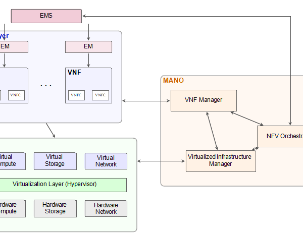
Table 4: Comprehensive Summary of Mathematical Notation in VNF-P
| Symbol | Description (Physical & Virtual Network) | Symbol | Description (Traffic Requests & Multi-Stage Graph) |
|---|---|---|---|
| Physical Substrate Network | Traffic Request & Service Chains | ||
| G = (N, L) | Physical network topology (nodes N, links L) | R | Set of traffic placement requests |
| n ∈ N | Physical node in the network | r ∈ R | A single traffic request tuple |
| l ∈ L | Physical link connecting nodes ni and nj | sr ∈ N | Source node of traffic request r |
| Bl | Bandwidth capacity of physical link l | dr ∈ N | Destination node of traffic request r |
| Dl | Physical length of link l | br | Requested bandwidth capacity for traffic request r |
| Tl | Physical transmission delay of link l | τr | Maximum allowable latency/delay in the SLA for traffic request r |
| S | Set of available servers in the network | CSLAr | SLA penalty cost factor per unit of delay violation |
| s ∈ S | A physical server instance | Fr ∈ F* | Service Function Chain (SFC) requested by traffic request r |
| Virtual Network Functions (VNFs) & Resources | Multi-Stage Graph Modeling (Section VI) | ||
| F | Set of available VNF types | Gr = (Vr, Er) | Virtual multi-state multi-stage graph for request r |
| f ∈ F | A specific Virtual Network Function type | Vr,k | Virtual node stage index k ∈ {1, …, |Fr| + 2} |
| K | Set of resource types (CPU, RAM, storage) | Vr,1 = {sr} | Start stage containing the source node |
| Cs,k | Available capacity of resource k ∈ K on server s | Vr,|Fr|+2 = {dr} | Terminal stage containing the destination node |
| Df,k | Demand of resource k ∈ K to instantiate VNF f | Vr,k (k > 1) | Intermediate node stages composed of server candidate nodes |
| Clicf | License cost associated with utilizing VNF f | (vr,k, vr,k+1) | Virtual directed transition link from stage k to k + 1 |
| Cdep | Standard physical deployment cost per server activation | Pr | Selected feasible routing path for traffic request r |
| Decision Variables | |||
| xrfn | Binary variable: 1 if VNF f requested by traffic r is allocated at physical node n; 0 otherwise. | ||
| yrfs | Binary variable: 1 if VNF f requested by traffic r is allocated on server s; 0 otherwise. | ||
| zfs | Binary variable: 1 if VNF type f is active on server s; 0 otherwise. | ||
| usn | Binary variable: 1 if server s is active or installed at physical node n; 0 otherwise. | ||
| wrl | Binary variable: 1 if traffic request r utilizes physical link l; 0 otherwise. | ||
| ar | Binary variable: 1 if traffic request r is successfully placed and accepted; 0 otherwise (SLA reject). | ||
| us, ul | Binary variables indicating whether server s or physical link l is active/utilized; 0 otherwise. | ||
2.1. Network Functions Virtualization Infrastructure (NFVI)
The NFVI corresponds to the data plane, providing the necessary resources to execute network services. It uses general-purpose hardware (COTS) to create a virtualization environment. The NFVI is subdivided into three components:
- PhysicalInfrastructure Layer: Comprises general-purpose servers that provide computing (multi-core CPUs), storage (SSDs/HDDs), and networking (L2/L3 switches, NICs) capabilities [14].
- VirtualizationLayer: Positioned between the physical and virtual infrastructure, this software layer uses hypervisors (e.g., KVM, VMware ESXi) to allocate physical resources into isolated environments, like Virtual Machines (VMs). It manages dynamic mapping to ensure high portability across VMs [6, 15].
- Virtual Infrastructure Layer: Includes virtual compute (VMs provisioned by hypervisor APIs), virtual storage (virtualized SAN/NAS), and virtual networks (interconnecting VMs via virtual switches like Open vSwitch) [6].
Despite ETSI’s framework, providers often customize NFVI implementations to suit their network constraints and geographic distributions.
2.2. Management and Orchestration (MANO)
MANO acts as the control plane, managing the virtualized con-text within the NFV framework, including hardware orchestration and VNF lifecycles. It comprises three blocks:
- VNFOrchestrator (NFVO): Orchestrates NFVI resources and manages the lifecycle of multiple chained VNFs, calculating optimal service paths.
- VNF Manager (VNF-M): Manages specific VNF instances throughout their lifecycle (instantiation, scaling, termination).
- Virtualized Infrastructure Manager (VIM): Controls the NFVIresources (compute, storage, network) and establishes connectivity between network endpoints [4].
2.3. VNF Layer
The VNF layer corresponds to the application plane. It aims to implement Physical Network Functions (PNFs)—like firewalls or DHCP servers—as software-based VNFs running on COTS hardware. Each VNF is composed of multiple VNF Components (VNFCs) managed by an Element Management System (EMS). The EMS collaborates directly with the VNF-M to execute lifecycle management effectively. Chaining multiple VNFs across different locations forms a complete Service Function Chain (SFC) capable of replacing traditional, proprietary hardware appliances.
3. Related Work
The VNF Placement (VNF-P) problem is a critical research area aimed at reducing CapEx and OpEx while ensuring the QoS of network traffic. Over the years, multiple optimization approaches have been proposed to tackle this problem under different network conditions.
Existing works addressing the VNF-P problem can be broadly classified based on the number of objectives optimized and the resolution strategy employed. As shown in Table 3, approaches are divided into Single-objective, Multi-objective (two or three objectives), and Many-objective (four or more objectives). Furthermore, the optimization strategies can be categorized into Scalarization methods (such as Weighted Sum and Lexicographic order) and Pareto-based approaches.
While Single-objective and Multi-objective approaches have been extensively studied, Many-objective optimization (MaOO) applied to VNF-P remains largely unexplored, particularly when combined with Pareto-based dominance. Scalarization methods often require prior knowledge of the objective weights, which is not always feasible in dynamic environments. In contrast, Pareto-based approaches provide a set of trade-off solutions, empowering net-work operators to make informed decisions. As highlighted in Table 3, there is a clear gap in the literature regarding Many-objective Pareto-based solutions for VNF-P, which this work aims to address.
Table 2 details the most common objective functions found in the literature.
Table 2: Objective functions proposed in the literature for static VNF-P
| Function | Definition |
|---|---|
| f1 | Energy cost (USD) |
| f2 | Bandwidth consumption (Mbps) |
| f3 | Latency (ms) |
| f4 | Traffic charge (kb) |
| f5 | Installation costs (USD) |
| f6 | Total cost of resources (USD) |
| f7 | Resource fragmentation (USD) |
| f8 | Utilization cost of all network links (USD) |
| f9 | Maximum network link utilization (Mbps) |
| f10 | Licensing costs (USD) |
| f11 | SLO costs (USD) |
| f12 | Traveled distance (km) |
| f13 | Number of hops |
| f14 | Number of servers |
| f15 | Number of VNF instances |
| f16 | Effective network throughput (%) |
| f17 | Percentage of allocated VNFs (%) |
Table 3: Taxonomy of Optimization Approaches in VNF-P
| Objectives | Scalarization (Weighted Sum / Lexicographic) | Pareto-based |
|---|---|---|
| Single-objective (1) | [16], [17], [18], [19], [20], [21], [22], [23], [24], [25], [26], [27], [28], [29] |
N/A |
| Multi-objective (2-3) | [6], [30], [31], [5], [32], [33], [34], [35], [36], [37], [38], [39], [40], [41], [9], [8] |
[42], [2], [43], [44], [10] |
| Many-objective (≥ 4) | None | Our Work |
4. VNF-P Problem Statement
4.1. Mathematical Symbols in VNF-P
This section presents the mathematical notation formulated for the VNF-P problem, as summarized in Table 4. A NFV environment comprises an underlying physical structure and various virtual components. The environment is organized through a net-
work topology 𝐺 = (𝑁, 𝐸), where 𝑁 and 𝐸 represent the set of physical node set and links, respectively. Each link 𝑒 ∈ 𝐸 is as-sociated to a bandwidth capacity 𝐵𝑒, a physical length 𝐿𝑒 and a transmission delay 𝛶𝑒.
To simplify the mathematical model we consider associated
usage costs for every VNF 𝑣 ∈ 𝑉 , among we can cite:
- Licensingcost 𝜆𝐶𝑣,
- Deployingcost 𝛿𝐶,
- Processingdelay T𝑣,
- Resourcerequirements 𝑀𝑟𝑣.
In the VNF-P problem, a set of requests is provided, where each request 𝑡 ∈ 𝑇 is composed of a service function chain 𝑊𝑡, a source node 𝑜𝑡 ∈ 𝑁, a destination node 𝜔𝑡 ∈ 𝑁, the requested traffic band-
width 𝛽𝑡, the maximum allowed delay 𝛥𝑡, cost of failing to meet the
maximum delay requirement 𝜌𝐶𝑡, i.e., 𝑡 = (𝑜𝑡, 𝜔𝑡, 𝛽𝑡, 𝛥𝑡, 𝜌𝐶𝑡, 𝑊𝑡).
4.2. Basic example of a VNF-P solution
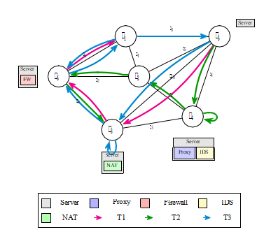
Consider a simple network topology for this practical example, as shown in Figure 2. The figure illustrates the placement of a service chain corresponding to two requests. The first request is depicted in green, with source node 𝑛1, destination node 𝑛5, and a
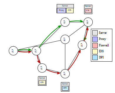
service chain comprising a Proxy deployed at node 𝑛7, an IDS at 𝑛7, and a Firewall at 𝑛8. Conversely, the second request, depicted in red, originates at node 𝑛1, terminates at node 𝑛8, and has a service chain comprising a DPI at node 𝑛4, an IDS at node 𝑛3, and a Firewall at node 𝑛8.
It is noteworthy that the different traffic flows utilize the Firewall located on the same server 𝑛8 without the need to instantiate it twice. It must be considered that when traffic traverses the links, it consumes bandwidth, and therefore, the physical capacity constraints of the links must be respected.
4.3. Multi/Many Objective Optimization Problems
The goal of a Multi-Objective Optimization Problem (MOOP) [45, 46] is to find a solution capable of simultaneously optimizing a set of objective functions while satisfying the defined constraints of the problem. Optimization implies either minimizing or maximizing an objective function; accordingly, a MOOP may require the minimization of certain objectives while simultaneously maximizing others.
A MOOP can be defined in a general manner as follows [46]:
\[
\begin{aligned}
&\underset{\mathbf{x}}{\text{Minimize/Maximize}}
&& f_m(\mathbf{x}),
&& m = 1,2,\ldots,M, \\[4pt]
&\text{subject to:}
&& g_j(\mathbf{x}) \geq 0,
&& j = 1,2,\ldots,J, \\[4pt]
&&& \mathbf{x} \in \mathbb{R}^{K}, \\[4pt]
&&& x_i^{L} \leq x_i \leq x_i^{U},
&& i = 1,2,\ldots,N.
\end{aligned}
\tag{1}
\]
A solution 𝑥 consists of a vector of N decision variables:
𝑥 = (𝑥1, … , 𝑥N). The value a decision variable can take lies be-tween a lower bound 𝑥𝐿 and an upper bound 𝑥𝑈 . These bounding restrictions constitute the decision space D.
The problem constraints consist of J inequalities and K equations, where 𝑔𝑗 (𝑥) and ℎ𝑘(𝑥) are referred to as constraint functions. The set of solutions that satisfy the J+K constraints and the 2N bounds is defined as the feasible region S, where D ⊆ S.
In a MOOP, there are M objective functions 𝑓(𝑥) = (𝑓1(𝑥), … , 𝑓M(𝑥)) that constitute a multidimensional space referred
to as the objective space Z, where each objective function represents either a minimization or a maximization problem. For each solution 𝑥 ∈ S, there is a corresponding point in the objective space,
denoted as 𝑓(𝑥) = 𝑧 = (𝑧1(𝑥), … , 𝑧M(𝑥)). Note that this maps an N-dimensional vector to an M-dimensional vector.
Finding a single optimal solution that simultaneously optimizes all objective functions in a MOOP is a fundamentally different task compared to single-objective optimization, due to the presence of conflicting objective functions. This leads to the existence of com-promise solutions, meaning that improving one objective function inevitably degrades another conflicting objective.
Without loss of generality, let us assume that all objective functions are to be minimized. In this context, given two solutions 𝑥, 𝑦 ∈ S, it is said that 𝑥 dominates 𝑦, denoted as 𝑥 ≻ 𝑦, if ∀𝑚 it holds that 𝑓𝑚(𝑥) ≤ 𝑓𝑚(𝑦) and ∃𝑚′ for which 𝑓𝑚′ (𝑥) < 𝑓𝑚′ (𝑦). In a MOOP, a set of mutually non-dominated solutions is called the Pareto Set, denoted as CP = {∀𝑥, 𝑦 ∈ S ∶ 𝑥 ⊁ 𝑦, 𝑦 ⊁ 𝑥}. The mapping of CP to the objective space Z is referred to as the Pareto Front, FP = {𝑧 = 𝑓(𝑥) ∶ 𝑥 ∈ CP} ⊆ Z. Specifically, the set of non-dominated solutions within the entire feasible region is defined as the Optimal Pareto Set CP∗ = {𝑥 ∈ S ∶ ∄𝑦 ≻ 𝑥}, and its corresponding mapping is the Optimal Pareto Front FP∗ = {𝑧 =𝑓(𝑥) ∶ 𝑥 ∈ CP∗} ⊆ Z. Note that for any given CP, it holds true that CP∗ ⪰ CP.
To illustrate this explanation, a two-dimensional graph can help visualize key concepts in MOOPs: the decision space, the objective space, the Pareto set, and the Pareto front. To construct the graph, random points are generated in the decision space and projected onto the objective space, highlighting the Pareto front.
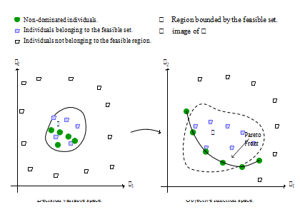
On the left side of Figure 3, the space representing the decision variables 𝑥 = (𝑥1, 𝑥2) is shown, with points representing the decision variable space. Feasible points are colored in light blue and green, which together form the feasible set 𝑆. The non-dominated points are highlighted in green. Finally, points that do not belong
to the feasible set are shown in pink.
On the right side, the objective space is depicted, where each point corresponds to 𝑓 = (𝑓1, 𝑓2) associated with the solutions from the decision space. The green points represent the Pareto Front (non-dominated solutions).
The size of the Optimal Pareto Set increases significantly as the number of objective functions grows, thereby increasing the complexity of the problem. In this regard, the literature distinguishes problems as low complexity if the MOOP considers two or three objective functions. However, if the number of objectives is greater than three, it is classified as a Many-Objective Optimization Problem (MaOP) [12].
4.4. Multi-Objective Formulation of the VNF-P Problem
Given an NFV environment defined by a topology 𝐺, a set of available physical servers 𝑆 in the network, a set of available VNFs 𝑉 , and a set of traffic requests 𝑇 , the VNF P problem seeks to compute a solution Θ that simultaneously minimizes the objective functions detailed in Table 2. This is formulated in the following expression:
\[
\mathbf{x} = (x_1, x_2, \ldots, x_n)
\tag{2}
\]
where 𝑀 = 17 and 𝑓𝑖 ∈ [0, ∞), subject to the available resource constraints on links and nodes.
The formulations and explanations of the objective functions are presented in equations (3) through (22), whereas the constraints are provided in equations (23) through (29).
4.5. VNF-P Problem Objective Functions
The objective functions to be optimized in the VNF-P problem can be classified into OPEX, CAPEX, and QoS levels, and they are defined as follows.
4.5.1. Energy Cost
This function calculates energy consumption across node de-vices such as routers and servers:
\[
Q_1 = Q_{1.1} + Q_{1.2}
\tag{3}
\]
where:
- 𝑓1.1is the energy consumption of the nodes to satisfy the traffic requests:
\[
Q_{1.1}
=
\sum_{n \in N}
\sum_{s \in S_n}
P_s x_{sn}
\tag{4}
\]
- 𝑓1.2is the energy consumption of the servers, calculated as:
\[
Q_{1.2}
=
\sum_{s \in S}
\mu_s
\left(
\left(P_s^{\max}-P_s^{\mathrm{idle}}\right)
\cdot
\frac{U_s^{\mathrm{CPU}}}{C_s^{\mathrm{CPU}}}
+
P_s^{\mathrm{idle}} \cdot x_s
\right)
\tag{5}
\]
- 𝑌𝑠is a binary variable, 1 if server 𝑠 is active, 0 otherwise,
- 𝑚𝑎𝑥𝑃𝑠is the maximum energy available on server 𝑠,𝑃𝑠is the energy consumed by server 𝑠 when idle,
- 𝑄𝑟𝑠is the quantity of computational resources 𝑟 = 𝑐𝑝𝑢 avail-able on server 𝑠, and𝑈𝑟𝑠 isthe quantity of computational resources 𝑟 = 𝑐𝑝𝑢 utilized on server 𝑠.
- 𝜏𝐶𝑛is the unitary energy consumption cost for the active physical node 𝑛,
- 𝑌𝑠is a binary variable, 1 if server 𝑠 is active, 0 otherwise,
- 𝜏𝐶𝑛is the unitary energy consumption cost for the active physical node 𝑛,
4.5.2. Bandwidth Consumption
This function computes the total bandwidth consumed across the network:
\[
Q_2
=
\sum_{l \in L}
b_l\,u_l
\tag{6}
\]
where 𝑢𝐵𝑒 is the bandwidth utilized on link 𝑒.
4.5.3. Latency
This function calculates the total traffic latency, which is gener-ated by link propagation delays and the processing delay of each VNF type deployed on the servers:
\[
Q_3
=
\sum_{r \in R}
\left(
\sum_{l \in L_r} d_l
+
\sum_{l \in L_r} T_l
\right)
\tag{7}
\]
where
- 𝛶𝑒is the data transmission delay on link 𝑒 utilized by traffic
𝑡, and
- T𝑣is the processing delay generated by VNF 𝑣.
4.5.4. Traffic Load
This objective function computes the traffic load by considering the operational cost of each active physical link, based on the delay and the total allocated bandwidth of the virtual links embedded within the physical link. In this work, the originally proposed distance variable found in the state of the art [33] was replaced by the delay variable.
\[
Q_4
=
\sum_{r \in R}
\mu_r
\left(
\sum_{l \in L}
\sum_{(i,j)\in E_r}
w_{rl}\, y_{ij}^{r}
\cdot
c_l
\right)
\tag{8}
\]
where
- 𝛶𝑛𝑛′is the propagation delay of a route segment between nodes 𝑛 and 𝑛′,
- 𝑋𝑡𝑣𝑛,𝑋𝑡𝑣′𝑛′ are binary variables, set to 1 if VNF 𝑣 (or 𝑣′) requested by traffic 𝑡 is allocated to the server connected to node 𝑛 (or 𝑛′), and 0 otherwise.
4.5.5. Installation Cost
This function computes the total installation cost for the servers plus the deployment cost for the VNFs:
\[
Q_{5}
=
\sum_{s \in S}
C_{s}^{\mathrm{inst}}\,x_{s}
+
\sum_{r \in R}
\sum_{f \in F_{r}}
C_{f}^{\mathrm{inst}}\,z_{rf}
\tag{9}
\]
where
- 𝛿𝐶𝑠is the deployment cost on server 𝑠,
- 𝜓𝐶𝑣is the unitary cost to deploy VNF 𝑣,
- 𝑊is the service function chain (SFC) requested by the traf-fics,
- 𝐴𝑡𝑣𝑠is a binary variable, 1 indicates that VNF 𝑣 from request
𝑡 is deployed on server 𝑠 ∈ 𝑆, 0 otherwise, and
- 𝑌𝑠is a binary variable, 1 indicates that server 𝑠 is active, 0
4.5.6. Total Resource Cost
This function calculates the cost of utilizing computational resources such as memory, CPU, and storage:
\[
Q_{6}
=
\sum_{n \in N}
\sum_{s \in S_n}
C_s \cdot x_{sn}
\tag{10}
\]
where
- 𝑈𝑟𝑠is the amount of computational resources of type 𝑟 utilized in server 𝑠, and
- 𝜅𝐶𝑟𝑠is the unitary cost of computational resource 𝑟 in server 𝑠.
To provide a realistic estimation of Operational Expenditures (OPEX) driven by resource utilization, the unitary cost parameters can be modeled after real-world public cloud pricing schemas, such as Amazon Web Services (AWS) Elastic Compute Cloud (EC2). For instance, an AWS EC2 m5.large instance (featuring 2 vCPUs and 8 GB of RAM) incurs a standard on-demand cost of approximately $0.096 per hour in the US East region. By translating these instance-level prices into unitary costs for individual compute and memory resources (𝜅𝐶𝑟𝑠), the objective function accurately reflects real monetary expenditures, thereby facilitating practical OPEX minimization in NFV deployments.
4.5.7. Resource Fragmentation
This function computes the cost of computational resources and bandwidth that have been allocated but remain unutilized:
\[
Q_{7}
=
\sum_{s \in S}
\mu_s
\sum_{k \in K}
\left(C_{sk}-U_{sk}\right)x_s
+
\sum_{l \in L}
\mu_l
\left(B_l-U_l\right)u_l
\tag{11}
\]
where:
- 𝑌𝑠is a binary variable, set to 1 if server 𝑠 is utilized, and 0 otherwise,
- 𝑌𝑒is a binary variable, set to 1 if link 𝑒 is utilized, and 0 otherwise,
- 𝑄𝑟𝑠is the quantity of computational resources of type 𝑟 available,
- 𝑈𝑟𝑠is the quantity of computational resources of type 𝑟 utilized in server 𝑠,
- 𝐵𝑒is the bandwidth available on link 𝑒,
- 𝑢𝐵𝑒is the bandwidth utilized on link 𝑒,
- 𝜎𝐶is the unitary cost for bandwidth underutilization, and
- 𝜙𝐶𝑟is the unitary cost for computational resource 𝑟 under-
4.5.8. Utilization Cost of All Network Links
This function computes the economic costs of the bandwidth utilized by traffic requests:
\[
Q_{8}
=
\sum_{l \in L}
u_l \cdot c_l
\tag{12}
\]
where
- 𝑢𝐵𝑒 is the bandwidth utilized on link 𝑒, and
- 𝛽𝐶𝑒is the unitary cost for the bandwidth of link 𝑒.
4.5.9. Maximum Utilized Network Link
This function calculates the link bearing the heaviest traffic load, as shown in the formula:
\[
Q_{9}
=
\max \left\{ u_l : l \in L \right\}
\tag{13}
\]
where 𝑢𝐵𝑒 is the bandwidth utilized on link 𝑒.
4.5.10. License Cost
This function computes the total sum of the license costs for both VNFs and servers:
\[
Q_{10}
=
\sum_{f \in F}
C_{f}^{\mathrm{lic}} \cdot z_f
+
\sum_{s \in S}
C_{s}^{\mathrm{lic}} \cdot x_s
\tag{14}
\]
where
- 𝑋𝑣𝑠 isa binary variable, set to 1 if VNF 𝑣 is allocated on server 𝑠, and 0 otherwise,
- 𝜆𝐶𝑣is the license cost of VNF 𝑣,
- 𝜂𝐶𝑠is the license cost of server 𝑠, and
- 𝑌𝑠is a binary variable, set to 1 if server 𝑠 is utilized, and 0
4.5.11. SLO Cost
This objective function calculates the penalty that must be paid to the client for Service Level Agreement (SLA) / Service Level Objective (SLO) violations:
\[
Q_{11}
=
\sum_{r \in R}
C_{r}^{\mathrm{SLA}}\,\delta_{r}
\tag{15}
\]
\[
\delta_{r}
=
\begin{cases}
D_{r}, & \text{if } D_{r} > \tau_{r},\\
0, & \text{otherwise}.
\end{cases}
\tag{16}
\]
where
- 𝜚𝐶𝑡is the penalty cost for an SLA violation for traffic 𝑡,
- 𝛥𝑡is the maximum allowed data transmission delay for traffic
- 𝐷𝑡is the total propagation delay for traffic 𝑡.
4.5.12. Distance Traveled
This function calculates the sum of the total distance traveled by the traffic requests:
\[
Q_{12}
=
\sum_{r \in R}
\sum_{l \in L_r}
D_l
\tag{17}
\]
where 𝐿𝑒 is the distance of link 𝑒.
4.5.13. Number of Hops
This function computes the total number of hops made by the traffic requests:
\[
Q_{13}
=
\sum_{r \in R}
h_r
\tag{18}
\]
where 𝑍𝑒 is an integer variable that counts the number of times traffic passes through link 𝑒.
4.5.14. Number of Servers
This objective function counts the number of servers utilized for VNF placement:
\[
Q_{14}
=
\sum_{s \in S}
x_s
\tag{19}
\]
where 𝑌𝑠 is a binary variable set to 1 if server 𝑠 is utilized, and 0 otherwise.
4.5.15. Number of VNF Instances
This function sums the quantity of deployed VNF instances:
\[
Q_{15}
=
\sum_{r \in R}
\sum_{f \in F_r}
z_{rf}
\tag{20}
\]
where 𝑋𝑠𝑣 is a binary variable set to 1 if VNF 𝑣 is allocated on server 𝑠, and 0 otherwise.
4.5.16. Effective Network Throughput
Given a list of traffic requests, this function aims to improve bandwidth utilization on each link by maximizing the ratio between accepted and rejected requests:
\[
Q_{16}
=
\frac{
\sum_{r \in R} b_r \cdot a_r
}{
\sum_{r \in R} b_r
}
\tag{21}
\]
- 5𝑡 is the requested bandwidth for traffic 𝑡, and
- 𝑌𝑡is a binary variable, 1 if traffic 𝑡 is placed within the net-work, 0 otherwise.
4.5.17. Percentage of Allocated VNFs
This function calculates the number of allocated VNFs re-quested by the traffic flows:
\[
Q_{17}
=
\frac{
\displaystyle \sum_{r \in R}
\sum_{f \in F_r}
\sum_{s \in S}
y_{rfs}
}{
\displaystyle \sum_{r \in R}
\sum_{f \in F_r}
1
}
\tag{22}
\]
where:
- 𝐴𝑡𝑣𝑠is a binary variable, 1 if VNF 𝑣 from traffic 𝑡 is deployed on server 𝑠, 0 otherwise, and
- 𝐻𝑡𝑣 isa binary constant, 1 if VNF 𝑣 is requested by traffic 𝑡, 0 otherwise.
4.6. VNF-P Problem Constraints
The VNF-P problem is subject to constraints at both the physical node and link levels, as well as at the virtual resource level, which are detailed below.
4.6.1. Server to Node Allocation
A server can only be allocated to a single node, expressed as follows:
\[
\sum_{s \in S_n} x_{sn} = 1,
\qquad \forall n \in N
\tag{23}
\]
where 𝑋𝑛𝑠 is a binary variable set to 1 if server 𝑠 is installed in node 𝑛, and 0 otherwise.
4.6.2. Server Resource Capacity
The sum of the resources utilized on a server must not exceed the total capacity of that server.
\[
d_{fk} \leq C_{sk},
\qquad \forall f \in F,
\qquad \forall s \in S
\tag{24}
\]
where:
- 𝑈𝑟𝑠represents the quantity of resources of type 𝑟 utilized in server 𝑠, 𝑈 = {𝑈𝑟𝑠 ∶ 𝑟 ∈ 𝑅, 𝑠 ∈ 𝑆}.
- 𝑄𝑟𝑠 representsthe quantity of computational resources of type 𝑟 available in server 𝑠, 𝑄 = {𝑄𝑟𝑠 ∶ 𝑟 ∈ 𝑅, 𝑠 ∈ 𝑆}.
4.6.3. VNF Resource Capacity
The sum of the resources utilized by a specific VNF type must not exceed the total capacity of the installed VNF of that same type available for reuse.
\[
b_r \leq B_l,
\qquad \forall r \in R,
\qquad \forall l \in L
\tag{25}
\]
where:
- 𝐾𝑟𝑣represents the quantity of resources of type 𝑟 utilized in
- 𝐽𝑟𝑣represents the quantity of available resources that the installed VNF can support, 𝐽 = {𝐽𝑟𝑣 ∶ 𝑟 ∈ 𝑅, 𝑣 ∈ 𝑉 }.
4.6.4. Bandwidth Capacity
The sum of the bandwidth utilized on a link must not exceed the available bandwidth of that link.
\[
D_r \leq \tau_r,
\qquad \forall r \in R
\tag{26}
\]
where:
- 𝐵𝑒is the bandwidth available on link 𝑒, 𝐵 = {𝐵𝑒 ∶ 𝑒 ∈ 𝐸}.
- 𝑢𝐵𝑒 is the bandwidth utilized on link 𝑒, 𝑢𝐵 = {𝑢𝐵𝑒 ∶ 𝑒 ∈.
4.6.5. NF Installation on Server
The resource demand of a VNF must not exceed the available capacity of the server where it is deployed.
\[
d_{fk}\, y_{rfs}
\leq
\left(C_{sk} – U_{sk}\right),
\qquad
\forall r \in R,\;
\forall f \in F_r,\;
\forall s \in S
\tag{27}
\]
where:
- 𝑈𝑟𝑠is the quantity of computational resources of type 𝑟 uti-lized in server 𝑠, 𝑈 = {𝑈𝑟𝑠 ∶ 𝑟 ∈ 𝑅, 𝑠 ∈ 𝑆}.
- 𝑄𝑟𝑠is the quantity of computational resources of type 𝑟 avail-able in server 𝑠, 𝑄 = {𝑄𝑟𝑠 ∶ 𝑟 ∈ 𝑅, 𝑠 ∈ 𝑆}.
- 𝑀𝑟𝑣is the computational resource requirement of type 𝑟 needed by VNF 𝑣, 𝑀 = {𝑀𝑟𝑣 ∶ 𝑟 ∈ 𝑅, 𝑣 ∈ 𝑉 }.
- 𝑋𝑣𝑠 isa binary variable, set to 1 if VNF 𝑣 is allocated on server 𝑠, and 0 otherwise.
4.6.6. VNF Reuse
The resource demand of the VNF type intended to be reused must not exceed the available capacity of the already installed VNF of the same type.
\[
b_r \cdot u_l
\leq
\left(B_l – U_l\right),
\qquad
\forall r \in R,\;
\forall l \in L
\tag{28}
\]
where:
- 𝐾𝑟𝑣is the quantity of computational resources of type 𝑟 uti-lized in the installed VNF 𝑣, 𝐾 = {𝐾𝑟𝑣 ∶ 𝑟 ∈ 𝑅, 𝑣 ∈ 𝑉 }.
- 𝐽𝑟𝑣is the quantity of available computational resources of type 𝑟 that the installed VNF 𝑣 can support, 𝐽 = {𝐽𝑟𝑣 ∶ 𝑟 ∈𝑅, 𝑣 ∈ 𝑉 }.
- 𝑀𝑟𝑣is the computational resource requirement of type 𝑟 that
VNF 𝑣 will reuse, 𝑀 = {𝑀𝑟𝑣 ∶ 𝑟 ∈ 𝑅, 𝑣 ∈ 𝑉 }.
the installed VNF 𝑣, 𝐾 = {𝐾𝑟𝑣 ∶ 𝑟 ∈ 𝑅, 𝑣 ∈ 𝑉 }.
- 𝐽𝑟𝑣represents the quantity of available resources that the installed VNF can support, 𝐽 = {𝐽𝑟𝑣 ∶ 𝑟 ∈ 𝑅, 𝑣 ∈ 𝑉 }.
- 𝑋𝑣𝑠 isa binary variable, set to 1 if VNF 𝑣 is allocated on server 𝑠, and 0 otherwise.
4.6.7. Traffic Bandwidth
The bandwidth requested by the traffic must not exceed the bandwidth available on the link:
\[
b_r \cdot u_{rl}
\leq
\left(B_l – U_l\right),
\qquad
\forall r \in R,\;
\forall l \in L
\tag{29}
\]
where:
- 𝐵𝑒 is the available bandwidth on link 𝑒.
- 𝑢𝐵𝑒 is the bandwidth utilized on link 𝑒.
- 𝑢𝐵𝑒is the utilized bandwidth on link 𝑒.
- 𝑋𝑡𝑒is a binary variable set to 1 if request 𝑡 utilizes link 𝑒, and 0 otherwise.
4.7. Numerical Example
This section introduces a basic example to elucidate the formulations provided in the preceding section. The problem instance is illustrated in Figure 4, and its input parameters are detailed in Tables 5 through 10.
Table 5 presents five VNF types in the rows, while the columns indicate costs (which are reference values in generic units) and associated characteristics. The VNF types, delay, deployment cost, license cost, bandwidth modification factor, required secondary memory, required number of cores, and required RAM are defined by 𝑉 , T, 𝜓𝐶, 𝜆𝐶, 𝛼𝛽, 𝑀𝑣 𝑟 , 𝑀𝑣 𝑟 , and 𝑀𝑣 𝑟 , respectively. The considered VNFs can be deployed on the same server depending on available capacity and requirements. Note that the Bandwidth Modification Factor column indicates the modification rate that the VNF exerts on the incoming traffic.
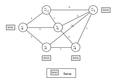
Table 5: Available VNF Parameters
| VNF | T | Parameter 1 | Parameter 2 | Parameter 3 | Resource 1 | Resource 2 | Resource 3 |
|---|---|---|---|---|---|---|---|
| f1 = Firewall | 20 | 10 | 50 | 1 | 30 | 4 | 8 |
| f2 = IDS | 12 | 9 | 45 | 1.3 | 35 | 6 | 8 |
| f3 = Proxy | 5 | 12 | 60 | 1.5 | 30 | 4 | 8 |
| f4 = NAT | 8 | 8 | 55 | 0.8 | 30 | 4 | 6 |
| f5 = DPI | 10 | 11 | 52 | 1.2 | 35 | 4 | 8 |
Table 6 presents the network link parameters. The rows display the bidirectional links, while the columns detail the set of links 𝐸, along with reference costs in generic units such as delay 𝜏, distance 𝐿, bandwidth usage cost 𝛽𝐶, and maximum link capacity 𝐵.
Table 7 presents the network node parameters. The columns display the set of nodes 𝑁, the set of servers 𝑆, and the energy cost 𝜏𝐶.
Table 6: Network Link Parameters
| Node | Parameter 1 | Parameter 2 | Parameter 3 | Parameter 4 |
|---|---|---|---|---|
| n1 | 7 | 690 | 0.14375 | 1000 |
| n8 | 9 | 1068 | 1.19E-05 | 1100 |
| n6 | 6 | 548 | 0.01223 | 1070 |
| n2 | 8 | 911 | 0.11931 | 1019 |
| n7 | 7 | 712 | 0.12741 | 1027 |
| n9 | 6 | 613 | 0.13651 | 1036 |
| n3 | 5 | 568 | 0.14531 | 1045 |
| n5 | 6 | 648 | 0.14561 | 1054 |
| n4 | 7 | 768 | 0.15471 | 1063 |
Table 7: Network Node Parameters
| Node | Connected Node | Parameter |
|---|---|---|
| n1 | – | 1.3E-4 |
| n2 | – | 1.3E-4 |
| n3 | n3 | 1.9E-4 |
| n4 | n4 | 1.0E-4 |
| n5 | n5 | 1.1E-4 |
| n6 | n6 | 1.4E-4 |
Table 8 presents the parameters for traffic requests 𝑡1, 𝑡2, and 𝑡3. The rows display each request 𝑡, while the columns outline their respective requirements. Each request is composed of a source node 𝑜, a destination node 𝜔, the requested bandwidth 𝛽, the maximum allowable delay without penalty 𝛥, the penalty cost for exceeding the maximum delay 𝜚𝐶, and the requested service chain 𝑊 . Furthermore, Table 9 presents the specific VNF requirements for these requests.
Table 10 presents the parameters of the available servers. This table details the set of servers 𝑆 alongside their reference costs in generic units, which include the license cost 𝜆𝐶, the deployment cost 𝛿𝐶, the maximum energy 𝑚𝑎𝑥𝑃 , the idle energy 𝑃 , the cost per core 𝜅𝐶𝑠𝑖 𝑟1 , the RAM cost 𝜅𝐶𝑠𝑖 𝑟2 , the storage cost 𝜅𝐶𝑠𝑖 𝑟3 , the number of available cores 𝑄𝑠𝑖 𝑟1 , the available RAM capacity 𝑄𝑠𝑖 𝑟2 , and the available external storage capacity 𝑄𝑠𝑖 𝑟3.
Table 8: Request Parameters
| Request | Source | Destination | Parameter 1 | Parameter 2 | Parameter 3 | Service Chain |
|---|---|---|---|---|---|---|
| r1 | n5 | n1 | 5 | 124 | 2 | v1 → v2 → v4 |
| r2 | n5 | n3 | 3 | 116 | 1 | v3 → v2 → v1 |
| r3 | n1 | n6 | 5 | 78 | 1 | v4 → v5 |
Table 9: VNFs Requested per Traffic
| VNF | n1 | n2 | n3 | |||
|---|---|---|---|---|---|---|
| RAM | CPU | RAM | CPU | RAM | CPU | |
| v1 | 2 | 3 | 2 | 4 | – | – |
| v2 | 2 | 4 | 2 | 3 | – | – |
| v3 | – | – | 2 | 3 | – | – |
| v4 | 1 | 2 | – | – | 2 | 3 |
| v5 | – | – | – | – | 1 | 3 |
Table 10: Server Parameters
| Node | Parameter 1 | Parameter 2 | Parameter 3 | Parameter 4 | Resource 1 | Resource 2 | Resource 3 | Capacity 1 | Capacity 2 | Capacity 3 |
|---|---|---|---|---|---|---|---|---|---|---|
| n3 | 85 | 2 | 2735 | 80 | 0.06 | 0.03 | 0.01 | 12 | 32 | 100 |
| n4 | 100 | 3 | 3000 | 100 | 0.07 | 0.04 | 0.02 | 12 | 32 | 106 |
| n5 | 110 | 2 | 3500 | 85 | 0.08 | 0.35 | 0.02 | 12 | 32 | 124 |
| n6 | 90 | 1 | 2735 | 94 | 0.075 | 0.048 | 0.01 | 12 | 32 | 130 |
An example solution is provided in Table 11, where the rows indicate the requests and the columns display the routing and place-ment for each requested VNF type. Figure 5 illustrates the solution graphically, depicting both the routing and the placement of the VNFs. The solutions for requests 𝑡1, 𝑡2, and 𝑡3 are the following, respectively:
- 𝑛5→ 𝑛3 → 𝑣1 → 𝑣2 → 𝑛6 → 𝑣4 → 𝑛1,
The same procedure applies to the other traffic requests: for 𝑡2, the accumulated delay is 65 time units, and for 𝑡3, it is 51 time units. The total accumulated delay for the set of traffic requests 𝑇 is 174 time units.Note that server 𝑠3 hosts functions 𝑣1 and 𝑣2, server 𝑠4 hosts functions 𝑣2 and 𝑣3, server 𝑠5 hosts function 𝑣5, and server 𝑠6 hosts functions 𝑣1 and 𝑣4, where 𝑣4 is reused by traffic requests 𝑡1 and 𝑡3. As observed in the solution, depending on the placement of the VNFs, it is possible for the path connecting a source and destination node pair to exhibit a cyclic structure. This implies resource overutilization in both links and nodes, as well as delays in traffic transfer. Consequently, this structure is significantly more complex than conventional routing.Based on the example in Figure 5, the following values can be observed:
- EnergyCost (𝑓1): For practical purposes, this function was divided into two operations. Operation 𝑓1.1 computes the sum of the energy costs utilized by passing through each node. Request 𝑡1 adds an energy cost of 00057 units for passing through the nodes, 𝑡2 adds 0.00068 units, and 𝑡3 adds 0.00084 units. In total, the energy cost for utilizing the nodes across all three requests is 0.00209 units. Operation 𝑓1.2 cal-culates the costs related to energy utilization in the servers.
- The amount of energy utilized is related to the number of active cores in the server multiplied by the energy cost. The sum of energy costs in servers 𝑠3, 𝑠4, 𝑠5, and 𝑠6 is 1.204715. The total energy cost (𝑓1.1 + 𝑓1.2) amounts to 1.206798332 units.
- BandwidthConsumption (𝑓2): The total bandwidth utilized across all links is 59.85 units.
- Latency (𝑓3):The accumulated delays for 𝑡1, generated within the links 𝐸𝑡 traversed by the traffic in the solution, are calculated by summing the following latency values: 𝑒5 = 6, 𝑒9 = 6, and 𝑒6 = 6, yielding a total of 18 units. Similarly, the processing delay for each VNF requested by 𝑡1 is summed: the delay for 𝑣1 is 20 time units, for 𝑣2 is 12 time units, and for 𝑣4 is 8 time units. Summing these yields a total of 40 time units for processing. Thus, the total delay for 𝑡1 is 18 (links) + 40 (processing), resulting in a total of 58 time units.
- Traffic Load (𝑓4): The traffic load is calculated by summing the product of the delay time and the bandwidth for each link between two servers hosting The load for 𝑡1 is calculated from node 𝑛3 (which hosts 𝑣1 and 𝑣2) to node 𝑛6 (which hosts 𝑣4), presenting a delay of 6 time units and a bandwidth
- 𝑛5
- Installation Cost(𝑓5): The sum of installation costs for the utilized servers 𝑠3, 𝑠4, 𝑠5, and 𝑠6 totals 8 On server 𝑠3, VNFs 𝑣1 and 𝑣2 were installed at a cost of 10 and 9 units, respectively. On server 𝑠4, the installed functions 𝑣2 and 𝑣3 sum a cost of 21 units. On server 𝑠5, 𝑣5 cost 11 units, and lastly, on 𝑠6, 𝑣1 and 𝑣4 were installed at a cost of 18 units. The sum of all VNF installation costs is 69 units, plus the server installation costs, yielding a total of 77 units.
- TotalResource Cost (𝑓6): On server 𝑠3, 10 cores, 16 RAM units, and 65 storage units were Multiplying these by their respective costs yields a total cost of 1.73 units for on link 𝑒9 equal to 6.5 units (considering the modification factor 𝛼𝛽). This results in 6 × 6.5, equaling 39 units. For 𝑡2 and 𝑡3, the result is 87.75 and 60 load units, respectively. Finally, the total sum of the products is 186.75 load units. 𝑠3. For 𝑠4, 𝑠5, and 𝑠6, the respective costs are 2.64, 1.3, and 2.76 units. The total cost of the utilized resources is 8.43 units.
- Resource Fragmentation (𝑓7): On server 𝑠3, 2 cores, 16 RAM units, and 35 storage units remained idle. Each unutilized resource is multiplied by its respective penalty cost, which are 0.0001 for cores, 0.0002 for RAM, and 0.0004 for storage. In summary, the penalty cost on 𝑠3 is 0.0174 units. For 𝑠4, 𝑠5, and 𝑠6, the penalty costs are 0.0198, 0.0412, and 0.0184 respectively, totaling 0.0968 units. This is subsequently added to the cost for not fully utilizing the bandwidth on each link, where a penalty of 0.0003 per unit applies. The total link penalty cost is 2.1927 units. The overall cost of the solution, summing the penalty costs across servers and links, is 2.289545 units.
- Utilization cost of all network links (𝑓8): For this function, the unitary bandwidth cost is multiplied by the bandwidth utilized on each The final result is 0.000104952 units.
- Maximum Network Link Utilized (𝑓9): This value represents the maximum bandwidth utilized among all network links, resulting in 17.15002 bandwidth units.
- LicenseCost (𝑓10): Two types of VNFs were installed on servers 𝑠 , 𝑠 , and 𝑠 . The license cost for each server plus the license cost for each installed VNF yields a total of 180, 205, and 195 units, respectively. On 𝑠5, a single VNF was installed, with a VNF license cost of 52 units, which, added to the server license cost, results in 162 units. The total cost for all licenses is 742 units.
- SLOCost (𝑓11): Each request is associated with a maximum allowable delay. If the request’s delay in the solution exceeds this defined maximum, the specific penalty cost for that re-quest is applied. For the solution in this example, no request exceeds the maximum delay; hence, this cost is 0.
- TraveledDistance (𝑓12): The sum of the distances traveled by each request is computed: 𝑡1 utilizes a route distance of 809, 𝑡2 utilizes 3.004, and finally, 𝑡3 totals 3.525 units. The total distance for the solution is 8.238 units.
- Numberof Hops (𝑓13): The total number of hops performed by each request across the links amounts to 12 units.
- Numberof Servers (𝑓14): 4 nodes were utilized to install the servers, resulting in a cost of 4 units.
- Numberof VNF Instances (𝑓15): The total number of VNF instances deployed on the servers reaches 7 units.
- Effective Network Throughput (𝑓16):In this example, all functions were successfully placed, resulting in a 100% effectiveness rate.
- Percentage of Allocated VNFs (𝑓17):In this example, all functions were successfully placed, yielding a rate of 100%.
In summary, by grouping the objective functions by type, a total OPEX cost of 8349.926 units, a total CAPEX cost of 742 units, and a total QoS cost of 379.900 units are obtained.
Table 11: Numerical example solution
| Request | Routing | VNF Placement | |||||
|---|---|---|---|---|---|---|---|
| n1 | n2 | n3 | n4 | n5 | n6 | ||
| r1 | n5, n3, n6, n1 | – | – | v1, v2 | – | – | v4 |
| r2 | n5, n4, n2, n6, n3 | – | – | – | v2, v3 | – | v1 |
| r3 | n1, n6, n1, n5, n3, n6 | – | – | – | – | v5 | v4 |
5. Multi-objective Evolutionary Algorithms
To address the formulation of the VNF-P problem based on the selected objectives, this work relies on Evolutionary Algo-rithms (EAs). Traditional Multi-Objective Evolutionary Algorithms (MOEAs) [45] are well-suited for problems with two or three objectives [47]. However, they suffer from significant scalability issues—such as loss of selection pressure, exponential increase in the proportion of non-dominated solutions, and computational overhead in diversity preservation—when the number of objectives grows [12]. This performance degradation motivates the use of Many-Objective Evolutionary Algorithms (MaOEAs) [48] for our VNF-P model considering the chosen set of objectives.
To manage the high dimensionality of the objective space, MaOEAs are generally grouped into families based on their diver-sity and selection mechanisms: decomposition-based approaches that optimize scalarizing sub-problems, relaxed dominance strategies (e.g., 𝜖- or 𝛼-dominance), indicator-based methods (e.g., hyper-volume), and objective reduction techniques. Algorithm 1 outlines the general evolutionary scheme shared by these algorithms.
Algorithm 1 General Scheme of MOEA/MaOEA
- Inputs: Evolutionary parameters and problems to solve
- Output: Pareto Set
- Begin:
- Initialize population P with N individuals
- Evaluate the objective functions and indicators for each individual in P
- While the stopping criterion is not met do:
- Select subsets of mating individuals
- Crossover mating individuals to generate new offspring
- Mutate the individuals generated by crossover
- Evaluate the objective functions and indicators for each individual
- Combine population P with the generated offspring
- Select the individuals that survive to the next generation
- Update population P
- End While
- Obtain the Pareto Set from P
- Return Pareto Set
- End
6. Evolutionary VNF-P
For the application of MOEAs, we define the chromosomal representation of the individual, the method for initializing the pop-ulation, the processes corresponding to the evolutionary operators (evaluation, selection, and crossover), and the input parameters of the algorithms. Figure 6 presents an example that correlates a solution, a chromosome structure, and the evaluation process.
6.1. Chromosome Structure
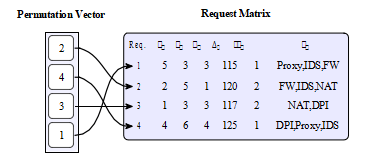
The chromosome structure is a permutation encoded in a vector whose size is equal to the number of requests to be processed. Each i-th position of the vector indicates the i-th traffic request for which the placement and routing must be calculated via a heuristic. A traffic request is represented by 𝑡 = (𝑜𝑡, 𝜔𝑡, 𝛽𝑡, 𝛥𝑡, 𝜌𝐶𝑡, 𝑊𝑡),while the set of requests 𝑡 is stored in a matrix. Figure 7 depicts a table comprising four requests, where each row stores the data corresponding to the requests 𝑡.
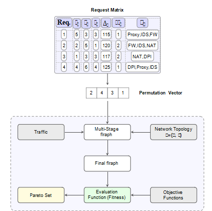
Furthermore, the 𝑖-th gene of the chromosome vector points to a row in the table where the 𝑖-th request to be processed is located. In the example provided in Figure 6, the chromosome vector [2,4,3,1] is observed, indicating that the requests defined in the table will be processed in that specific sequence.
6.2. Multi-stage Graph Modeling
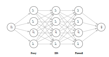
In this work, we extend the approach described in [49], where it is suggested that a traffic request 𝑡 = (𝑜𝑡, 𝜔𝑡, 𝛽𝑡, 𝛥𝑡, 𝜌𝐶𝑡, 𝑊𝑡) be mapped onto a virtual directed multi-stage graph. This virtualgraph consists of |𝑊𝑡| + 2 stages, where |𝑊𝑡|denotes the length of the service chain 𝑊𝑡. The first stage 𝐸1 comprises the source node𝑜𝑡, whereas the final stage consists of the destination node 𝜔𝑡, i.e.,𝐸1 = {𝑜𝑡}, 𝐸|𝑊𝑡|+2 = {𝜔𝑡}.Each intermediate stage 𝐸𝑖 (𝑖 ∈{2, …,(|𝑊𝑡| + 1)}), is composed of physical nodes featuring candidate servers for placing the 𝑗-th VNF, with 𝑗 = 𝑖 – 1. Evidently, these servers must possess available computational resources to host the VNF. For each pair of nodes 𝑛𝑗 ∈ 𝐸𝑖 and 𝑛𝑘 ∈ 𝐸𝑖+1, a virtual link (𝑛𝑗 ,𝑛𝑘) is added between them. Finally, once the multi-stage graph is constructed, it is verified whether at least one valid path exists from the source node 𝑜𝑡 to the destination node 𝜔𝑡. A valid path will not exist if at least one of the intermediate stages is an empty set. Figure 8 presents the final structure of the multi-stage graph corresponding to the original network topology and traffic 𝑡2.Formally, for a given traffic request 𝑡, the multi-stage graph is defined as a directed graph 𝐺̂𝑡 = (𝑉̂ , 𝐴̂𝑡). The set of vertices 𝑉̂ is the union of all stages, i.e., 𝑉̂𝑡𝑡⋃|𝑊 |+2𝑖=1𝑡𝐸𝑖. The set of arcs 𝐴̂𝑡 consists of directed virtual links connecting nodes in adjacent stages. An arc (𝑛𝑗 , 𝑛𝑘) ∈ 𝐴̂𝑡 exists if and only if 𝑛𝑗 ∈ 𝐸𝑖, 𝑛𝑘 ∈ 𝐸𝑖+1 (for some 1 ≤ 𝑖 ≤ |𝑊𝑡| + 1), and there is a feasible physical path from 𝑛𝑗 to 𝑛𝑘 in the underlying network 𝐺 satisfying the bandwidth requirement 𝛽𝑡.Algorithm 2 formalizes the multi-stage graph construction procedure described above.
Algorithm 2 Multi-Stage Graph Construction
Require:
Traffic request r = (sr, dr, br, τr,
CSLAr, Fr),
physical graph G = (N, L), resource state A
Ensure:
Multi-stage graph
Ĝr = (V̂r, Êr),
or INFEASIBLE
- V1 ← {sr};
V|Fr|+2 ← {dr} - for k ← 2 to |Fr| + 1 do
- i ← k – 1
{i-th VNF to host: Fr[i]} - Vk ←
{n ∈ N :
server at n has sufficient residual resources for Fr[i]} - if Vk = ∅ then
- return INFEASIBLE
- end if
- end for
- Êr ← ∅
- for k ← 1 to |Fr| + 1 do
- for each
vk ∈ Vk,
vk+1 ∈ Vk+1
do - if ∃ path
vk → vk+1
in G with residual bandwidth ≥ br
then - Êr ←
Êr ∪
{(vk, vk+1)} - end if
- end for
- end for
- return
Ĝr =
(⋃k Vk, Êr)
6.3. VNF Placement
A solution is defined as the placement of a VNF in each of the intermediate stages of the multi-stage graph. It should be re-called that there are as many intermediate stages as there are VNFs required by the corresponding traffic request.To install the 𝑗-th VNF on a server in stage 𝑖 (where 𝑗 = 𝑖-1), the impact of its installation is evaluated across each of the servers in that stage. This impact is associated with a metric calculated after installing the VNF on the server. Ultimately, the server exhibiting the lowest impact measure is selected.To compute the impact following the installation of the 𝑗-th VNF on the servers of stage 𝑖, the values of the objective functions are first calculated. Subsequently, each of these values is normalized. Afterwards, the normalized values are summed and divided by the total number of objective functions, thereby yielding an average cost for each server. Finally, the servers in stage 𝑖 are sorted from lowest to highest based on this cost and stored in a list according to this order.The procedure for server selection at each stage constitutes a greedy constructive heuristic. At each step, it chooses the server that presents the lowest impact cost, provided that both the server and the physical link to this stage are available. If both resources are enabled, the VNF is installed on the selected server, and the process advances to the next stage of the multi-stage graph. It important to note that an exact shortest-path algorithm (e.g., Dijk-stra’s algorithm) cannot be directly applied to the multi-stage graph because the arc costs (impact scores) are dynamically dependent on the continuously updating residual resource state A.In the event that the required server or link is unavailable, alter-natives are considered by evaluating the next server with the lowest cost on the ranked list. If no viable options are found in the current stage, a backtracking mechanism retreats to the previous stage in order to explore alternative routes.If, after exhausting all possible local combinations via back-tracking, a valid route cannot be established, the heuristic terminates and it is concluded that a feasible solution for the corresponding traffic request cannot be found.Physical routing between selected servers is constructed sequentially from the source to the destination, traversing the nodes of each stage and the nodes of the selected shortest-path link in the underlying physical topology.Algorithms 3 and 4 formalize these two procedures. Finally, the solution obtained in the multi-stage graph for traffic 2 is depicted in Figure 9, while its representation in the original graph is illustrated in Figure 10. The final solution, which reflects the result of the entire process after placing traffic 1, traffic 2, and traffic 3, is captured in Figure 11. The routing of the final solution is determined as follows:– Traffic 1: 𝑛5, 𝑛3, 𝑛6, 𝑛1– Traffic 2: 𝑛5, 𝑛4, 𝑛2, 𝑛6, 𝑛3– Traffic 3: 𝑛1, 𝑛6, 𝑛1, 𝑛5, 𝑛3, 𝑛6It is worth noting that the apparent cycle in the routing of Traffic 3 (e.g., visiting node 𝑛1 and 𝑛6 twice) is intentional and strictly valid within the multi-stage NFV model. A physical node can host VNFs that structure cycles or self-loops, allowing it to be visited repeatedly to satisfy complex intermediate routing and placement needs.The model independently accounts for computational resources during VNF placement and link bandwidth consumption during physical traversal, natively supporting non-simple paths when they represent the most cost-effective or feasible global placement.
Algorithm 3 VNF Impact Function
Require:
Server s, VNF index i, resource state A, objectives
f1, …, fm,
bounds fjmin, fjmax
Ensure:
Impact score impact(s) ∈ [0, 1]
- Hypothetically install Fr[i] on s
(temporarily update A) - for j ← 1 to m do
- Evaluate fj(s) under the hypothetical placement
- f̂j(s) ←
fj(s) – fjmin
fjmax – fjmin
- end for
- Restore A (undo hypothetical installation)
- return
impact(s) =
(1 / m)
∑j=1m
f̂j(s)
Algorithm 4 Greedy VNF Placement with Backtracking
Require:
Multi-stage graph Ĝr, physical graph G, resource state A
Ensure:
Placement P = (p1, …, p|Fr|) and route R,
or UNPLACED
- k ← 2;
P ← 〈〉;
R ← 〈sr〉 - L[k] ← [],
q[k] ← 1 for all stages k
{Ranked server lists and pointers} - while k ≤ |Fr| + 1 do
- i ← k – 1
- if L[k] is empty then
- Compute impact(s) for each s ∈ Vk (Algorithm 3)
- L[k] ← sort Vk by impact(·) ascending;
q[k] ← 1 - end if
- placed ← false
- while q[k] ≤ |L[k]| do
- s ← L[k][q[k]];
q[k] ← q[k] + 1 - if
s has resources for Fr[i]
and
∃ path R.last() → s with bandwidth ≥ br
then - Install Fr[i] on s (update A);
P ← P ‖ 〈s〉 - Append shortest path R.last() → s to R
- placed ← true;
break - end if
- end while
- if not placed then
- if k = 2 then
- return UNPLACED
{Cannot backtrack beyond first stage} - end if
- Undo installation of Fr[i – 1] from P.last()
(restore A) - P.pop(); Remove last segment from R;
L[k] ← [] - k ← k – 1
{Backtrack to previous stage} - else
- k ← k + 1
- end if
- end while
- if
∃ path R.last() → dr in G
with bandwidth ≥ br
then - Append shortest path R.last() → dr to R
- return (P, R)
- end if
- return UNPLACED
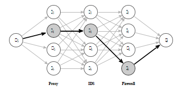
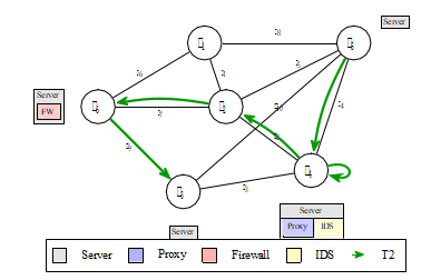
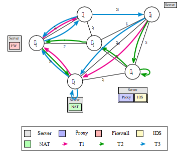
6.4. Constraint Handling and Feasibility
A critical aspect of many-objective optimization is the treatment of constraints, which in the VNF-P problem are governed by Equations (23) through (29) (covering physical node and link capacity constraints such as CPU, memory, storage, bandwidth, and max-imum latency limits). Rather than employing traditional exterior penalty functions—which can severely distort the objective space and hinder convergence in many-objective environments—this work implements a hybrid of Constrained Encoding and an active Repair Mechanism integrated directly within the multi-stage decoding process.Specifically, the following three mechanisms are applied:
- ConstrainedEncoding (Active Filtering): During the construction of the virtual multi-stage graph for each traffic re-quest (defined in Section 6-B), candidate physical nodes and links are filtered A physical server is only included as a candidate in stage 𝐸𝑖 if it has sufficient residual CPU, memory, and storage capacity to host the 𝑗-th VNF. Similarly, physical links are only included as candidate transitions if their available bandwidth meets the request demand. This prevents the generation of structurally invalid individuals.
- Active Repair and Backtracking: When selecting a path across the multi-stage graph, if a stage is reached where no candidate servers can satisfy the resource constraints, or if the linking physical paths violate the accumulated latency limit, the algorithm triggers a backtracking This mechanism undoes the placement in the previous stage 𝐸 𝑖−1 and attempts to route through the next best-ranked feasible candidate.
- Feasible Space Projection:If all combinations are ex-hausted and a traffic request cannot be routed under the strict constraints of physical nodes and links, the request is flagged as unplaced (contributing to a penalty in the throughput and Service Level Objective (SLO) cost objectives), but the chro-mosome’s structure remains mathematically valid. For example, in highly congested scenarios such as the INDIA35 topology with Traffic_600 or the Zib54 topology with Traffic_3000 (Saturated loads), empirical observations indicate an infeasibility (unplaced request) rate of approximately 10% to 25% even after the repair mechanism is exhausted. By simply dropping these requests rather than creating invalid configurations, the structure guarantees that the decoded physical mapping strictly complies with network
Through this hybrid approach, every chromosome decoded always maps to a feasible execution state in the physical network without requiring external penalty factors, ensuring that the evolutionary search is restricted to the strictly feasible region of the solution space.
7. Pareto Performance Metrics
In this study, metrics were utilized to measure the characteristics of the known Pareto front (PFK) relative to a true Pareto front (PFT). Since no single metric can capture all characteristics, they are briefly explained below [45, 50, 51]:
- GenerationalDistance (GD): GD is an indicator that reports how far, on average, PFK is from PFT. This indicator can be mathematically defined as:
\[
GD :=
\frac{1}{H}
\left(
\sum_{f \in PFK}
\left(
\operatorname{dist}(f,PFT)
\right)^p
\right)^{\frac{1}{p}}
\tag{30}
\]
where:
- His the number of vectors in PFK,
- dist(f,PFT) is the phenotypic distance between the vec-tor 𝑓 ∈ PFK and PFT, that is:
\[
\operatorname{dist}(f,PFT)
=
\min_{f^{*}\in PFT}
\left\{
\operatorname{dist}\!\left(f,f^{*}\right)
\right\}
\tag{31}
\]
If GD = 0, then PFK = PFT. In this study, we consider p = 2 in accordance with [52], thus the distance is Euclidean.
- Inverted Generational Distance (IGD): This indicator mea-sureshow far, on average, PFT is from PFK. In this study, the following indicators were utilized, mathematically defined as:
\[
\mathrm{IGD}
:=
\frac{1}{\left|PF^{T}\right|}
\left(
\sum_{p^{*} \in PF^{T}}
\operatorname{dist}\left(p^{*},PF\right)^q
\right)^{\frac{1}{q}}
\tag{32}
\]
where 𝐶 is the number of vectors in PFT and p = 1 in accordance with [52]. If IGD = 0, then PFK = PFT.
- Epsilon Indicator (𝐼𝜖 ): Given PFK and PFT, the additive 𝐼𝜖 defines the minimum value 𝜖 ∈ ℝ such that any vector in PFT is 𝜖-dominated by at least one solution in PFK.
\[
I_{\epsilon}
=
\min
\left\{
\epsilon \in \mathbb{R}
\;\middle|\;
\forall f^{*}\in FPT,\;
\exists f\in FPK
\text{ such that }
\forall i\in\{1,\ldots,\alpha\},
\;
f_i^{*}\leq f_i+\epsilon
\right\}
\tag{33}
\]
where 𝛼 indicates the number of objective functions of the problem. If 𝐼𝜖 > 0, then PFK must be moved by at least 𝜖 units to completely dominate PFT. If 𝐼𝜖 = 0, then every solution in PFT is dominated or equaled by some solution in PFK.
- Maximum Pareto Front Error (ME): This metric mea-sures how well one set of vectors compares with another. This metric can be mathematically expressed as:
\[
\mathrm{ME}
:=
\max_{p \in PF}
\left\{
\min_{p^{*} \in PF^{T}}
\left\{
\operatorname{dist}\left(p,p^{*}\right)
\right\}
\right\}
\tag{34}
\]
More specifically, it measures the largest minimum distance between each vector in PFK and the corresponding closest vector in PFT.
- Spacing(S): This metric numerically describes the spread of the vectors in PFK, which can be mathematically described as:
\[
S
:=
\left(
\frac{1}{|PF|-1}
\sum_{p \in PF}
\left(
d(p,PF)-\bar{d}
\right)^2
\right)^{\frac{1}{2}}
\tag{35}
\]
where
- 𝑑𝑖𝑠𝑡(𝑓,𝑃 𝐹 𝐾) is the closest distance from vector 𝑓 to the set PFK-{f } whose structure is identical to Equation (31).
- 𝑑𝑖𝑠𝑡is the average distance of the vectors, that is:
When S = 0, all vectors are evenly spaced. As the uniformity deteriorates, S increases. In this study p = 2 in accordance with [52].
- 𝑅𝑘Indicator: Given that the exact hypervolume calculation is #P-hard in general [53], and even practical state-of-the-art sweeping algorithms (such as WFG or those based onnKlee’s measure problem [54, 55]) exhibit a worst-case time complexity bounded by U(𝜂 log 𝜂 + 𝜂𝛼∕2) for 𝛼 ≥ 3 (where 𝜂 size of the PFK set (U(𝐾 ⋅ |𝑃 𝐹 𝐾| ⋅ 𝛼)).
These indicators are based on the concept of aggregate utility functions applied to a collection of preference directions uniformly distributed over the simplex. Each variant represents a different way of evaluating the utility of the set, allowing for flexible and computationally efficient assessment.𝑅𝑘 indicator can be mathematically expressed as:
\[
R_k
=
\frac{1}{\left|PFK\right|}
\sum_{\lambda^{j}\in\Lambda}
\min_{f\in PFK}
u_k\!\left(f,\lambda^{j}\right)
\tag{36}
\]
where,
- Λ is a set of weight vectors uniformly generated over the simplex Δ𝛼−1, that is: Λ = {𝜆(1), … , 𝜆(𝐾)} with
𝑖 𝑖(𝑗)𝛼 ∑𝛼(𝑗)(𝑗)
- 𝑢𝑘(𝑓,𝜆𝑗 ) is a scalarizing function that reduces the vec-tor 𝑓 to a numerical value.
In this context, the literature proposes three 𝑅𝑘-type indica-tors: 𝑅1, 𝑅2, and 𝑅3. These quality indicators are explained below.
- 𝑅1Indicator: This indicator utilizes an additive utility function (Linear Weighted Sum) that averages the performance of the PFK under multiple linear preferences, making it suitable for convex problems. This utility can be mathematically expressed as:
\[
u_1\!\left(f,\lambda^{j}\right)
=
\sum_{i=1}^{\alpha}
\lambda_i^{j}\cdot f_i
\tag{37}
\]
- 𝑅2 Indicator: Introduces a Chebyshev-type utility func-tion (Weighted Tchebycheff) relative to an ideal point, emphasizing the worst weighted deviation. Mathematically, this utility can be expressed as:
\[
u_2\!\left(f,\lambda^{j}\right)
=
\max_{1\leq i\leq \alpha}
\left\{
\lambda_i^{j}\cdot
\left|f_i-z_i^{*}\right|
\right\}
\tag{38}
\]
where 𝑧∗ = {𝑧∗, … , 𝑧∗} is a reference or ideal point. 8.2. Objective Function SelectionThis indicator is more sensitive to vectors with poor per-formance in at least one objective, and is more robust against non-convex fronts.
- R3 Indicator: This indicator evaluates the degree of coverage of the set with respect to each preference di-rection, utilizing an inverse and normalized function. This is expressed mathematically as:
\[
H_{3}\!\left(Q^{i},Q^{*}\right)
=
\max_{1 \leq j \leq m}
\left[
\frac{1}{w_j}
\cdot
\frac{q_j^{i}-q_j^{*}}
{q_j^{U}-q_j^{L}}
\right]
\tag{39}
\]
Table 12: Traffic Load Classification
| Traffic Load | Effective Transfer Rate |
|---|---|
| Low | 75 – 100% |
| Medium | 45 – 74% |
| High | 20 – 44% |
| Saturated | 0 – 19% |
8. Computational Experiments
The simulations conducted in this section seek to answer two questions: (1) Which objective functions should be considered in the problem as a MaOP, and (2) What is the performance of the implemented MaOEAs? In this context, we initially present the computational environment utilized for the tests; subsequently, tests are conducted to determine the correlation between objective functions and consequently discard redundant ones. Finally, simulations are performed in order to compare the performance of the implemented MaOEAs.
8.1. Computational Environment
The computational simulations were carried out in a con-trolled environment, utilizing a Lenovo Legion Y540-15IRH laptop, equipped with an Intel Core i7-9750H processor (6-core, 12-thread architecture, with a 2.6 GHz base frequency and 4.5 GHz maxi-mum turbo frequency), 16 GB of DDR4 RAM, and a 1 TB Solid State Drive (SSD) as primary storage. The operating system em-ployed was Microsoft Windows 10. The evolutionary algorithms were implemented using the MOEAFramework library in Java [52]. Each execution was performed sequentially on a single thread, without employing multi-core parallelism, to guarantee result repro-ducibility and avoid variations associated with concurrency. These specifications allowed for the efficient execution of multiple runs of the evolutionary algorithms without incurring significant hard-ware limitations or performance penalties during the evaluation, selection, and solution generation processes. It is worth noting that the same evolutionary parameters previously defined in the corresponding section were maintained, with the aim of preserving methodological homogeneity and ensuring the comparability of the results obtained across the different experimental scenarios.
8.2. Objective Function Selection
Feature selection, as a dimensionality reduction technique, aims to select a subset of relevant features from the original ones by elim-inating redundant features. This generally leads to an improved performance of the evolutionary process, that is, better Pareto front quality and lower computational cost [56]. In this study, the elimination of redundant objective functions was considered given that all are deemed relevant.To construct the vector set 𝐹 , we first evaluate the solutions obtained across preliminary simulations utilizing NSGA-III over the 12 scenarios. Data vectors of the 17 metrics are collected awhere 𝑧𝑛𝑎𝑑 = (𝑧𝑛𝑎𝑑 , … , 𝑧𝑛𝑎𝑑 ) is the nadir point. This variant is particularly useful for capturing both the con-vergence and diversity of the vectors.the final generation, obtaining a substantial sample of 2400 observations (100 solutions per 24 scenarios). The first step calculates the Pearson correlation (𝑟) between pairs of functions. Additionally, the coefficient of determination (𝑟2) is utilized to quantify the level of redundancy, indicating what percentage of the variance of one function is explained by the other. If two pairs of functions 𝑓𝑎 and 𝑓𝑏 have a correlation equal to or greater than 80% (𝑟2 > 0.64), one of them is a candidate to be eliminated. A sensitivity analysis revealed that thresholds of 75%, 80%, and 85% produce exactly the same subset of 𝑀 = 11 objective functions, demonstrating robustness. Lowering the threshold to 70% is too aggressive, discarding additional functions where more than half of their variance is independent information, whereas raising it to 90% retains too many redundant objectives, failing to alleviate the many-objective complexity [57, 12]. Furthermore, discarding decisions are not merely statistical; domain knowledge plays a crucial role. For instance, evaluating performance metrics and navigating the search space in 17 dimensions is mathematically complex and computationally expensive, often exacerbating the curse of dimensionality. Specifically, in such high-dimensional spaces, the proportion of non-dominated solutions grows exponentially, leading to dominance resistance, where traditional Pareto-based selection completely loses selection pressure. While the many-objective algorithms utilized in this work (e.g., MOEA/D and NSGA-III) are explicitly designed to cope with dominance resistance by relying on reference-based decomposition and scalarization instead of pure Pareto dominance, discarding highly correlated, domain-redundant objectives still critically alleviates computational bottlenecks and preserves the physical significance of the optimization process.Tables 13 and 14 summarize the sensitivity analysis for objective reduction. The thresholds 75%, 80%, and 85% yield an identical subset of 𝑀 = 11 objective functions, indicating stability within a range of ±5 percentage points around the 80% threshold.Lowering the threshold to 70% discards 𝑓10 and 𝑓12, corresponding to the CAPEX and distance coverage. On the other hand, a threshold of 90% retains 14 objectives, providing an insufficient reduction. Therefore, the 80% threshold provides an adequate balance between removing redundant functions and preserving the fundamental criteria of the problem.
8.2.1. Test Instances and Experimental Scheme
The objective function selection procedure was carried out through the following steps:
- Aset of 𝑁𝑒𝑠𝑐 = 24 scenarios is considered.
Table 13: Discard Table – Complete Sensitivity Analysis
| Selected Function | Discarded Function | ρ | Minimum Threshold |
|---|---|---|---|
| |ρ| ≥ 90% | |||
| f7 Resource fragmentation | f14 Number of servers | 99% | 90% |
| f2 Bandwidth consumption | f8 Link utilization cost | 99% | 90% |
| f16 Effective transfer rate | f17 Percentage of allocated VNFs | 94% | 90% |
| 85% ≤ |ρ| < 90% | |||
| f10 License cost | f5 Installation cost | 88% | 85% |
| f1 Energy cost | f14 Number of servers | 87% | 85% |
| f12 Distance traveled | f13 Number of hops | 86% | 85% |
| f1 Energy cost | f6 Total resource cost | 86% | 85% |
| 80% ≤ |ρ| < 85% – chosen threshold in the thesis | |||
| f10 License cost | f6 Total resource cost | 84% | 80% |
| 75% ≤ |ρ| < 80% – no new pair with both functions active | |||
| f3 Latency | f13 Number of hops (already discarded) | 79% | – |
| f5 Installation cost (already discarded) | f6 Total resource cost (already discarded) | 78% | – |
| 70% ≤ |ρ| < 75% – pairs with both functions active at 80% | |||
| f1 Energy cost | f10 License cost | 74% | 70% |
| f3 Latency | f12 Distance traveled | 73% | 70% |
| f2 Bandwidth consumption | f13 Number of hops (already discarded) | 72% | – |
| f8 Link utilization cost (already discarded) | f13 Number of hops (already discarded) | 71% | – |
| f10 License cost | f14 Number of servers (already discarded) | 71% | – |
Table 14: Sensitivity Analysis Summary for Objective Reduction
| Threshold | Discarded | Retained (m) | Discarded Functions |
|---|---|---|---|
| 90% | 3 | 14 | f8, f14, f17 |
| 85% | 6 | 11 | f5, f6, f8, f12, f14, f17 |
| 80% – chosen | 6 | 11 | f5, f6, f8, f12, f14, f17 |
| 75% | 6 | 11 | f5, f6, f8, f12, f14, f17 |
| 70% | 8 | 9 | f5, f6, f8, f10, f12, f13, f14, f17 |
- Each scenario 𝑖 is configured according to a network topology, a traffic load (with a set of requests in an all-to-all scheme), and the blocking type.
- For each scenario 𝑖, 𝑁𝑠𝑜𝑙 = 100 consistent solutions Θ𝑖 ={Θ𝑖1, … , Θ𝑖𝑁𝑠𝑜𝑙 } are calculated.
- For each solution Θ𝑖𝑗 , the objective function vector 𝐹 ={𝑓1, … , 𝑓𝑀} is calculated.
- With ⋅ 𝑁n𝑠𝑜𝑙 solutions Θ 𝑖𝑗, the Pearson correlation is computed for each pair (𝑓𝑎, 𝑓𝑏) of objective functions.
The experimental tests were conducted on three network topologies with distinct characteristics regarding the number of nodes and links: NSF [58], depicted in Figure 12; EON-RT [59], in Figure 13; and INDIA35 [60], in Figure 14. The links in these topologies present an average bandwidth varying between 1000 and 1200 Mbps, while the servers feature, on average, 64 CPU cores, 128 GB of RAM, and 1200 GB of storage.
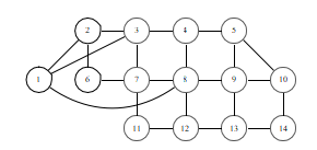
In each topology, multiple executions were performed utilizing different traffic request loads, classified into four levels: Low,computed for each pair (𝑓𝑎, 𝑓𝑏) of objective functions.The experimental tests were conducted on three network topologies with distinct characteristics regarding the number of nodes and links: NSF [58], depicted in Figure 12; EON-RT [59], in Figure 13; and INDIA35 [60], in Figure 14. The links in these topologies present an average bandwidth varying between 1000 and 1200 Mbps, while the servers feature, on average, 64 CPU cores, 128 GB of RAM, and 1200 GB of storage.In each topology, multiple executions were performed utilizing different traffic request loads, classified into four levels: Low, Medium, High, and Saturated. These loads were designed to force scenarios with blockages in links and/or servers, allowing the evaluation of the system’s behavior under congestion conditions.In the experiment, two types of blocking were considered:
- Node blocking: the available resources in the links were considerably increased to prevent rejections due to lack of capacity in them, ensuring that request blockages were exclusively caused by insufficient server resources.
- Link blocking: the computational resources of the servers (CPU,RAM, and storage) were increased so that any request rejection was due solely to the lack of capacity in the links.
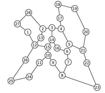
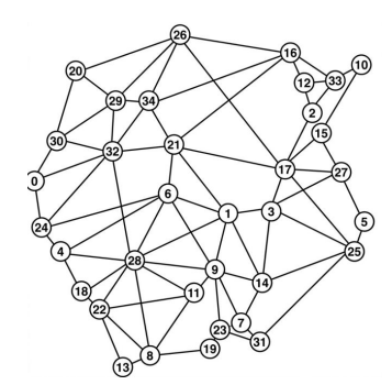
Table 15 summarizes all the test scenarios, classified according to the blocking type, the topology utilized, the load level applied in each execution, and the average effective transfer rate (throughput) corresponding to each load for each blockage. The bandwidth and number of VNFs columns are explained below. To adequately con-figure the test conditions, the following adjustments were made to the traffic requests:
- In the case of link blocking, the initial required bandwidth was modified in order to induce an average rejection rate that permitted classifying the load into the aforementioned
- In the case of node blocking, the number of VNFs per request was adjusted to cause rejections due to a lack of resources in the servers, also allowing their classification into Low, Medium, High, and Saturated.
For each of the topologies, a set of traffic requests was generated following an all-to-all scheme, that is, from all nodes to all other nodes in the network. Under this scheme, the NSF topology generated 182 requests, while EON-RT and INDIA35 produced 756 and 1190 requests, respectively. These experiments identified the loads corresponding to the four congestion levels for both types of blocking.
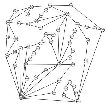
8.2.2. Results and Discussions
Table 16 presents the results of the correlation analysis be-tween pairs of objective functions. If the correlation is greater than 80% between two objective functions, it implies low contradiction, whereby one of the functions is eliminated to avoid redundancy.Finally, Table 17 displays the comparisons made between highly correlated objective functions.
8.3. Objective Functions Discarding Justification
To reduce the dimensionality of the Many-Objective Problem (MaOP) and avoid redundancy, highly correlated objective functions (over 80% correlation) were analyzed to determine which should be retained and which discarded, as detailed in Table 17. The elimination decisions were strictly guided by the physical meaning and operational relevance of each objective within the NFV environment:
- InstallationCost (𝑓5): It presented an 88% correlation with License Cost (𝑓10). 𝑓10 was retained because license fees are recurring and more representative of the continuous software based nature of VNFs, whereas the installation is usually a one-time deployment expense.
- TotalResource Cost (𝑓6): It was highly correlated with both Energy Cost (𝑓1, 86%) and License Cost (𝑓10, 84%). Since 𝑓1 and 𝑓10 already provide a detailed account of the operational and software expenditures respectively, maintaining 𝑓6
Table 15: Test Scenario Configuration Table
| Network | Load | Bandwidth Blocking | Node Blocking | ||
|---|---|---|---|---|---|
| Throughput | Bandwidth (Mb/s) | Throughput | Number of VNFs | ||
| NSF | Low | 89.005 | 25 | 89.65 | 2 |
| Medium | 52.19 | 65 | 46.115 | 4 | |
| High | 19.5 | 200 | 18.385 | 10 | |
| Saturated | 7.965 | 600 | 6.455 | 25 | |
| EON-RT | Low | 93.645 | 4 | 93.675 | 1 |
| Medium | 61.7 | 9 | 49.765 | 2 | |
| High | 19.77 | 50 | 19.315 | 5 | |
| Saturated | 6.415 | 150 | 7.62 | 11 | |
| INDIA35 | Low | 82.835 | 15 | 79.505 | 1 |
| Medium | 57.515 | 25 | 41.74 | 2 | |
| High | 15.625 | 150 | 16.345 | 5 | |
| Saturated | 7.775 | 300 | 7.605 | 10 | |
Table 16: Pearson correlations between objective functions
| f1 | f2 | f3 | f4 | f5 | f6 | f7 | f8 | f9 | f10 | f11 | f12 | f13 | f14 | f15 | f16 | f17 | |
|---|---|---|---|---|---|---|---|---|---|---|---|---|---|---|---|---|---|
| f1 | 41% | 57% | 42% | 66% | 86% | -8% | 41% | 7% | 74% | 3% | 41% | 48% | 87% | 18% | -52% | -53% | |
| f2 | 61% | 43% | 19% | 30% | -52% | 99% | 26% | 19% | 12% | 62% | 72% | 29% | 10% | -44% | -43% | ||
| f3 | 65% | 28% | 55% | -34% | 61% | 17% | 28% | 14% | 73% | 79% | 40% | 19% | -83% | -88% | |||
| f4 | 25% | 42% | -19% | 43% | 13% | 24% | 22% | 33% | 39% | 35% | 17% | -69% | -73% | ||||
| f5 | 78% | -2% | 19% | 1% | 88% | -4% | 17% | 18% | 47% | 32% | -25% | -27% | |||||
| f6 | -13% | 30% | 7% | 84% | 0% | 32% | 36% | 48% | 28% | -53% | -56% | ||||||
| f7 | -51% | -15% | 5% | -4% | -32% | -39% | 99% | 15% | 23% | 23% | |||||||
| f8 | 25% | 19% | 12% | 61% | 71% | 28% | 10% | -44% | -43% | ||||||||
| f9 | 1% | 2% | 14% | 18% | 7% | 2% | -11% | -11% | |||||||||
| f10 | -2% | 20% | 21% | 71% | 32% | -27% | -29% | ||||||||||
| f11 | 14% | 15% | 3% | 1% | -10% | -11% | |||||||||||
| f12 | 86% | 24% | 12% | -43% | -45% | ||||||||||||
| f13 | 27% | 11% | -52% | -54% | |||||||||||||
| f14 | 48% | -41% | -41% | ||||||||||||||
| f15 | -18% | -20% | |||||||||||||||
| f16 | 94% | ||||||||||||||||
| f17 | |||||||||||||||||
would introduce redundancy in OPEX evaluation. Therefore,𝑓6 was discarded.
- Utilization Cost of All Network Links (𝑓8):It showed an almost perfect correlation (99%) with Bandwidth Consumption (𝑓2). 𝑓2 provides a more direct and universally understood metric of network traffic volume in NFV, making 𝑓8 expendable.
- Number of Hops (𝑓13):It exhibited an 86% correlation with Distance Traveled (𝑓12). While hops represent logical distances, 𝑓12 reflects the physical geographic propagation distance which has a more direct impact on signal latency. Thus, 𝑓13 was discarded.
- Numberof Servers (𝑓14): It showed high correlations with Energy Cost (𝑓1, 87%) and Resource Fragmentation (𝑓7, 99%). Energy consumption (𝑓1) is inherently driven by the number of active servers, making 𝑓14 Retaining 𝑓1 and 𝑓7 better captures both the environmental impact and the efficiency of server utilization.
- Percentage of Placed VNFs (𝑓17):It correlated strongly (94%) with Network Effective Transfer Rate (𝑓16, Through-put). In service provider environments, throughput (𝑓16) is a much more critical performance indicator for user satisfaction and Quality of Service (QoS) than the mere percentage of successfully instantiated VNFs. Consequently, 𝑓17 was eliminated.
As a result of this analysis, 11 relevant objective functions were selected, namely: Energy Cost (𝑓1), Bandwidth Consumption (𝑓2), Latency (𝑓3), Load Traffic (𝑓4), Resource Fragmentation (𝑓7), Maximum utilized network link (𝑓9), License Cost (𝑓10), SLO Cost (𝑓11), Distance Traveled (𝑓12), Number of VNF instances (𝑓15), and Network effective transfer rate (𝑓16).
Table 17: Discard Table
| O.F.1 | O.F.2 | Correlation % | Discarded O.F. |
|---|---|---|---|
| f10 License cost | f5 Installation cost | 88% | f5 Installation cost |
| f1 Energy cost | f14 Number of servers | 87% | f14 Number of servers |
| f7 Resource fragmentation | f14 Number of servers | 99% | f14 Number of servers |
| f2 Bandwidth consumption | f8 Utilization cost of all network links | 99% | f8 Utilization cost of all network links |
| f12 Distance traveled | f13 Number of hops | 86% | f13 Number of hops |
| f16 Network effective transfer rate | f17 Percentage of placed VNFs | 94% | f17 Percentage of placed VNFs |
| f1 Energy cost | f6 Total resource cost | 86% | f6 Total resource cost |
| f10 License cost | f6 Total resource cost | 84% | f6 Total resource cost |
8.4. MaOEA Performance Analysis
These simulations were conducted considering the eleven objective functions selected in the previous section, assessing threeMaOEAs: R-VEA [61], MOEA/D [62], and NSGA-III [63]. These MaOEAs are widely recognized for their efficacy in MaOPs.
8.4.1. Evolutionary Parameters
The configuration applied to the MaOEAs included the type of genetic operators, population size, and stopping criteria, selected to ensure a fair comparison among them.
Genetic Operators:
All algorithms employed Polynomial Mutation [47] as the mutation operator, with a mutation probability of 𝑝𝑚 = 1∕𝐿 (where 𝐿 is thenumber of decision variables) and a distribution index of 𝜂𝑚 = 20.0.Regarding the crossover operator, R-VEA and NSGA-III applied the Simulated Binary Crossover (SBX) [64] operator with a crossover probability of 𝑝𝑐 = 1.0 and a distribution index of 𝜂𝑐 = 30.0, whereas MOEA/D utilized the Differential Evolution (DE) [65] operator with a crossover rate of 𝐶𝑅 = 1.0 and a scaling factor of 𝐹 = 0.5. The relatively high SBX distribution index (𝜂𝑐 = 30) controls the dispersion of offspring, generating children closer to their parents to favor finer local search [63].In all three algorithms, parent selection was performed randomly, aiming to preserve the genetic diversity of the population during the evolutionary process.
Population Size:
To maintain homogeneous experimental conditions, the population size was fixed at 90 individuals for the three considered algorithms (R-VEA, MOEA/D, and NSGA-III). In the cases of R-VEA and NSGA-III, this value emerges naturally from the generation of reference points utilizing outer divisions = 2 and inner divisions = 1, according to the MOEAFramework implementation and following the provisions of their respective original works [61], [63].Let 𝛼 be the number of objectives and 𝐻 the number of di-visions. The number of reference points generated by a layer is obtained by:
\[
\eta(\alpha,H)
=
\binom{\alpha+H-1}{H}
=
\binom{\alpha+H-1}{\alpha-1}
\tag{40}
\]
When two layers are employed (𝐻𝑜𝑢𝑡𝑒𝑟 = 2 and 𝐻𝑖𝑛𝑛𝑒𝑟 = 1), the target population size is calculated as:
\[
\eta
=
\eta(\alpha,H_{\mathrm{outer}})
+
\eta(\alpha,H_{\mathrm{inner}})
\tag{41}
\]
\[
\eta
=
\binom{\alpha+H_{\mathrm{outer}}-1}{H_{\mathrm{outer}}}
+
\binom{\alpha+H_{\mathrm{inner}}-1}{H_{\mathrm{inner}}}
\tag{42}
\]
Particularly, for 𝛼 = 12 objectives, we have:
\[
\eta_{1}
=
\binom{12+2-1}{2}
=
\binom{13}{2}
=
78
\tag{43}
\]
\[
\eta_{2}
=
\binom{12+1-1}{1}
=
\binom{12}{1}
=
12
\tag{44}
\]
which results in a total population size of 𝜂 = 90.Both R-VEA and NSGA-III employ this same combinatorial scheme, although in R-VEA it is often expressed in terms of 𝛼 − 1 instead of 𝐻, an equivalent notation in the literature. In the case of MOEA/D, the MOEAFramework defaults to a population of 100 individuals. However, in this work, it was adjusted to 90 to ensure a fair comparison.
Stopping Criterion:
To control the execution duration and allow a fair comparison among the MaOEAs, the simulation adopts the maximum number of generations fixed at 𝑀𝑎𝑥𝐺𝑒𝑛 = 300 as the stopping criterion,which is equivalent to 𝑁𝐹 𝐸 = 𝑃𝑜×𝑀𝑎𝑥𝐺𝑒𝑛 = 90×300 = 27, 000Number of Function Evaluations per execution. This was determined from a preliminary experiment aimed at analyzing the con-vergence behavior of the NSGA-III algorithm. In that experiment,the Zib54 network topology with 2000 traffic requests was utilized, along with Generational Distance (GD) as the metric recorded every 50 generations. The results showed that starting from generation 250-300, the GD value stabilized without significant improvements.
8.4.2. Test Instances
For the test instances, the network topologies Zib54 [66] depicted in Figure 15, EON-RT [59] in Figure 13, and INDIA35 [60] in Figure 14 were utilized. The number of requests corresponding to the Low, Medium, High, and Saturated load levels was calculated previously for each topology, following the scale defined in Table 12. These values are detailed in Table 18. In total, twelve experimental scenarios were defined, in which traffic requests were generated randomly. Recall that each request is composed of the following tuple 𝑡 = (𝑜𝑡, 𝜔𝑡, 𝛽𝑡, 𝛥𝑡, 𝜌𝐶𝑡, 𝑊𝑡). In this regard, each component was selected according to the following schemes:
- 𝑜𝑡= traffic origin is randomly generated among all network nodes.
- 𝜔𝑡= traffic destination is randomly generated among all net-work nodes.
- 𝛽𝑡= minimum traffic bandwidth at the source node is gener-ated in a range between two and five Mbps [40].
- 𝛥𝑡= maximum allowable delay is equal to twice the delay from source to destination under low traffic load.
- 𝜌𝐶𝑡= penalty cost in dollars for exceeding the delay declared in the SLA is between one and two dollars.
- 𝑊𝑡 = number of VNFs per traffic request is generated be-tween two and four VNFs.
Considering these criteria, we proceed to perform the simulations explained in the following subsection.
Table 18: Test Scenarios
8.4.3. Experimental Scheme
| Topology | Load | # Requests |
|---|---|---|
| Zib54 | Low | 600 |
| Zib54 | Medium | 1000 |
| Zib54 | High | 2000 |
| Zib54 | Saturated | 3000 |
| India35 | Low | 400 |
| India35 | Medium | 600 |
| India35 | High | 1000 |
| India35 | Saturated | 2000 |
| EON | Low | 300 |
| EON | Medium | 500 |
| EON | High | 980 |
| EON | Saturated | 1500 |
The experimental scheme is the overall process for performing evolutionary simulations, obtaining Pareto fronts, and calculating performance metrics. The scheme is explained below:
- Aset of 𝑁𝑒𝑠𝑐 = 12 scenarios was defined, each determined by a combination of a network topology and a traffic load level.
- Foreach scenario, a number f of traffic requests was generated according to the corresponding load, see Table 18.
- EachMaOEA was executed independently for each scenerio.
- To mitigate the effect of stochastic variability inherent to evolutionary algorithms and obtain statistically representative estimations, each algorithm was executed 𝑁𝑒𝑗= 30 times per scenario independently using different random seeds, as recommended in the literature for reliable estimation of average performance and variability. Consequently, the total number of executions performed in the study was 𝑁𝑒𝑗 × 𝑁𝑎𝑙𝑔 × 𝑁𝑒𝑠𝑐 = 30 × 3 × 12 = 1, 080 independent executions.
- Asa result, 𝑁𝑒𝑗 = 30 Pareto fronts were obtained for each scenario and algorithm combination.
- To evaluate algorithm performance, the quality metrics de-finedin Section 7 were applied to the Pareto fronts obtained in each execution.
At the end of these steps, statistical calculations were performed presenting the performance of the MaOEAs according to the traffic scenario and quality metrics. The figures and their discussions are provided in the following subsection.
8.4.4. Results and Discussion
Before presenting Figure 16, recall that the value of each cell, for each topology and load combination (low, medium, high, and saturated), corresponds to the average over 𝑁𝑒𝑗 = 30 Pareto fronts calculated in that scenario, as mentioned in the previous section.Figure 16 summarizes the performance of the multi-objective algorithms by topology and load, reporting quality metrics (GD, IGD, 𝐼𝜀, ME, S, 𝑅1, 𝑅2, 𝑅3). The horizontal blocks correspond to the topologies and the vertical blocks to the different traffic load levels (low, medium, high, and saturated). Each block displays subcolumns corresponding to the evaluated algorithms (NSGA-III, MOEA/D, and R-VEA), and the rows indicate the performance metrics (GD, IGD, ME, S, R1, R2, and R3) employed to compare the results.Each cell shows the average value of the metric from 𝑁𝑒𝑗 = 30 Pareto fronts generated in that same scenario (same topology and same load).Except for 𝑅1, which is maximized, all metrics (GD, IGD, 𝐼𝜀, ME, 𝑆, 𝑅2, and 𝑅3) are minimized: lower values are better.The shaded cells mark the best value within the corresponding scenario (same topology and load), comparing algorithms. For instance, if in the ZIB54 topology and saturated load the IGD cell for NSGA-III displays 3.234𝐸 − 01 and is shaded, it indicates that the average (over 𝑁𝑒𝑗 = 30 fronts) IGD obtained by NSGA-III in that scenario is 3.234𝐸 − 01, and that this value is the best (lowest) compared to the other evaluated algorithms in ZIB54 with saturated load.Table 19 presents a detailed numerical comparison of the three evaluated MaOEAs—NSGA-III, MOEA/D, and R-VEA—across the three network topologies (ZIB54, INDIA35, and EON-RT) and four traffic load levels (Low, Medium, High, and Saturated). Shaded cells indicate the best-performing algorithm for each topology-load combination according to each metric. Several patterns emerge from this analysis. First, R-VEA dom-inates GD and ME across virtually all scenarios: it achieves a GD of 0 (perfect convergence) in nearly every ZIB54 and INDIA35 scenario, indicating that its approximated Pareto front contains at least one solution that coincides with the reference front. A similar
Table 19: Performance metrics comparison across topologies and traffic loads. Shaded cells indicate the best-performing algorithm per scenario
| Topology | Metric | Low Load | Medium Load | High Load | Saturated Load | ||||||||
|---|---|---|---|---|---|---|---|---|---|---|---|---|---|
| NSGA-III | MOEA/D | R-VEA | NSGA-III | MOEA/D | R-VEA | NSGA-III | MOEA/D | R-VEA | NSGA-III | MOEA/D | R-VEA | ||
| ZIB54 | GD | 0.0138 | 0.0134 | 0 | 0.0156 | 0.0174 | 0 | 0.0157 | 0.0166 | 0 | 0.0156 | 0.0172 | 0 |
| IGD | 0.2976 | 0.3345 | 0.6642 | 0.3210 | 0.3628 | 0.7401 | 0.3140 | 0.3613 | 0.6967 | 0.3234 | 0.3769 | 0.7815 | |
| HV | 0.3505 | 0.3528 | 0.6948 | 0.3515 | 0.4059 | 0.7052 | 0.3554 | 0.3974 | 0.6969 | 0.3352 | 0.4383 | 0.7717 | |
| ME | 0.3111 | 0.2644 | 0 | 0.3512 | 0.3056 | 0 | 0.3375 | 0.2870 | 0 | 0.3339 | 0.3087 | 0 | |
| S | 30622 | 38850 | 0 | 39744 | 45838 | 0 | 30087 | 55247 | 2344 | 31652 | 44088 | 0 | |
| f1 | 1.37e-03 | 1.37e-03 | 1.37e-03 | 1.37e-03 | 1.37e-03 | 1.37e-03 | 1.37e-03 | 1.37e-03 | 1.37e-03 | 1.37e-03 | 1.37e-03 | 1.37e-03 | |
| f2 | 1518702 | 1490606 | 1492719 | 1513905 | 1490978 | 1490271 | 1500451 | 1472352 | 1461464 | 1498792 | 1472926 | 1471190 | |
| INDIA35 | GD | 0.0174 | 0.0163 | 0 | 0.0170 | 0.0175 | 0 | 0.0174 | 0.0185 | 0 | 0.0162 | 0.0182 | 0 |
| IGD | 0.3204 | 0.3518 | 0.6753 | 0.3203 | 0.3528 | 0.6696 | 0.3404 | 0.3812 | 0.6919 | 0.3323 | 0.3739 | 0.7143 | |
| HV | 0.3429 | 0.3903 | 0.7628 | 0.4030 | 0.4283 | 0.7944 | 0.3820 | 0.4223 | 0.9288 | 0.3649 | 0.4709 | 0.7787 | |
| ME | 0.3445 | 0.2952 | 0 | 0.3457 | 0.3062 | 0 | 0.3776 | 0.3168 | 0 | 0.3593 | 0.3136 | 0 | |
| S | 4166 | 4357 | 4658 | 3941 | 5519 | 0 | 3380 | 4903 | 511.9540 | 3923 | 5319 | 1199 | |
| f1 | 1.37e-03 for all algorithms and load levels | ||||||||||||
| f2 | 104874 | 103873 | 104331 | 103026 | 101338 | 101567 | 104731 | 102245 | 102837 | 105164 | 102937 | 103254 | |
| EON-RT | GD | 1.69e-03 | 0 | 0 | 3.14e-03 | 0 | 0 | 2.65e-03 | 0 | 0 | 0 | 0 | 0 |
| IGD | 0.2753 | 0.3154 | 0.6516 | 0.2743 | 0.3180 | 0.6945 | 0.2811 | 0.3286 | 0.6300 | 0.2910 | 0.3449 | 0.7130 | |
| HV | 0.3848 | 0.5127 | 0.7789 | 0.3193 | 0.4171 | 0.6997 | 0.3867 | 0.4000 | 0.6494 | 0.3320 | 0.4255 | 0.7621 | |
| ME | 0.1446 | 0 | 0 | 0.2078 | 0 | 0 | 0.1906 | 0 | 0 | 0 | 0 | 0 | |
| S | 2111 | 2943 | 1493 | 2255 | 3069 | 2853 | 2467 | 3502 | 1853 | 2634 | 2838 | 1264 | |
| f1 | 1.37e-03 for all algorithms and load levels | ||||||||||||
| f2 | 59650 | 58344 | 58709 | 57086 | 55200 | 55418 | 58089 | 56528 | 57564 | 59824 | 58029 | 58261 | |
trend is observed for the Maximum Pareto Error (ME), where R-VEA systematically achieves ME= 0, confirming that no member of its front lies significantly far from the reference. This behavior is expected, as R-VEA’s angle-penalized distance mechanism is specifically designed to maintain reference-point convergence. Second, NSGA-III consistently achieves the best IGD and 𝐼𝜀 values across all topologies and loads. For example, in ZIB54 under low load, NSGA-III obtains IGD= 0.2976 compared to MOEA/D’s 0.3345 and R-VEA’s 0.6642. This advantage holds across all four load levels and all three topologies, indicating that NSGA-III generates a more uniformly spread approximation front that covers the objective space more comprehensively. The consistently higher IGD and 𝐼𝜀 of R-VEA suggests that, while it achieves good point wise convergence (low GD), its front is less diverse and covers fewer regions of the Pareto front.Third, behavior under the Spacing (S) metric is topology-dependent. In ZIB54 (a large backbone network), R-VEA achieves the best spacing in most scenarios, producing a more evenly dis-tributed front. In INDIA35 (a medium-sized national topology), results are more balanced: NSGA-III leads under low load, while R-VEA leads under medium and saturated conditions. In EON-RT (a compact optical network), R-VEA and NSGA-III alternate as the best performers, suggesting that topology size and connectivity density influence which algorithm achieves better solution spacing.Fourth, the 𝑅2 indicator—a weighted utility metric—favors MOEA/D or R-VEA depending on the topology. In ZIB54, MOEA/D obtains the best 𝑅2 under low load, while R-VEA leads under high and saturated loads. In INDIA35 and EON-RT, MOEA/D consistently obtains the lowest 𝑅2 values, suggesting better alignment with the reference weight vectors in smaller, more structured topologies. The 𝑅1 indicator, which is identical across all algorithms in all scenarios (≈ 1.37 × 10⁻³), reflects that all three algorithms produce fronts of comparable quality when measured by this particular weighted indicator, and therefore does not discriminate between them.Overall, the results in Table 19 confirm the complementary nature of the three algorithms: R-VEA excels in convergence (GD, ME), NSGA-III excels in coverage and diversity (IGD, 𝐼𝜀), and MOEA/D achieves competitive 𝑅2 performance especially on smaller topologies. These findings are consistent with the aggregate best-count analysis presented in subsequent figures.Figure 17 summarizes what is detailed in Figure 16. Figure 17 takes those values cell-by-cell and, for each metric, counts in how many scenarios each algorithm achieved the best result. It is observed that R-VEA maintains the best values in GD and ME, con-firming better convergence capacity, whereas NSGA-III achieves the best results in IGD and Iε, evidencing superior convergence toward the optimal Pareto front and a broader coverage/diversity of solutions. MOEA/D places with an intermediate performance, standing out for its global consistency across most metrics. This figure allows for clearly identifying the particular strengths of each algorithm: R-VEA in convergence, NSGA-III in diversity, and MOEA/D as a balanced solution.Figure 18 analyzes the behavior of the algorithms under different network load conditions (low, medium, high, and saturated). Similarly to the section on Figure 17, the number of times an algorithm had the best performance according to the load level is counted. In low load scenarios, differences between algorithms are minor, given that the network has sufficient resources and VNF placement does not present significant conflicts. As the load in-creases, differences become more noticeable: R-VEA maintains superior stability, preserving a well-defined Pareto front even under saturation conditions. NSGA-III, while retaining good solution dispersion, shows greater variability and lower precision in convergence. MOEA/D, for its part, achieves competitive results at low loads, but its performance decreases slightly in saturation scenarios due to its lower search space exploration capacity.Figure 19 summarizes the global performance count of the number of times the three algorithms (NSGA-III, MOEA/D, and R-VEA) achieved the best result, considering the ZIB54, INDIA, and EON topologies. It is observed that algorithm behavior varies notably depending on the evaluated network structure.
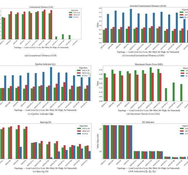
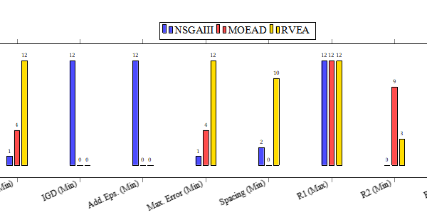
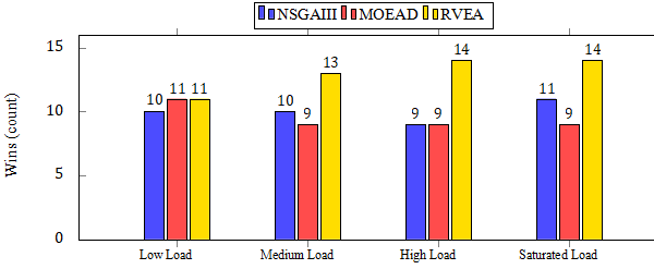
In the ZIB54 topology (large network), the R-VEA algorithm demonstrates clearly superior performance, reaching the highest number of favorable metrics (22), whereas NSGA-III and MOEA/D obtain more modest performances (12 and 6, respectively). In the case of the INDIA topology (medium size), all three algorithms present a more balanced behavior: NSGA-III obtains 13 metrics, alongside R-VEA with 15 and MOEA/D with 12, suggesting a tighter competition. Finally, in the EON topology (small network), the best performance corresponds to MOEA/D with 20 metrics, followed by NSGA-III and R-VEA, both with 15.These results reflect that there is no single dominant algorithm across all topologies, but rather their effectiveness depends on the structural characteristics of each network. In particular, R-VEA excels in larger networks like ZIB54, while MOEA/D benefits in more compact topologies such as EON.Figure 20 presents a comparative performance summary by algorithm, integrating the average values of all analyzed metrics and scenarios. The graph allows for clearly visualizing the overall superiority of R-VEA, which combines precise convergence and balanced diversity, outperforming the other approaches in most eval-uated contexts. R-VEA accumulates 52 cases (≈ 40%), followed by NSGA-III with 40 (≈ 30.8%) and MOEA/D with 38 (≈ 29.2%).These results consolidate the trend shown in previous figures: R-VEA is the most consistent method by obtaining the highest number of victories across metrics and topologies, while NSGA-III and MOEA/D exhibit a competitive and proximate performance to each other.
8.5. Execution Time Analysis
The execution times recorded for each network topology and traffic load scenario are summarized in Table 20. The results reveal two consistent trends. First, execution time is strongly influenced by the topology size: the Zib54 topology (54 nodes) required between 6 and 7 times more computation than EON-RT (28 nodes). Second, within the same topology, variations across traffic load levels are moderate (generally below 20%), indicating that structural network size has a larger impact on execution time than traffic volume.R-VEA was consistently the most computationally efficient algorithm across all topologies and load levels. On average, NSGA-III required approximately 6–11% more time than R-VEA, making both algorithms comparable and suitable for practical deployment scenarios. MOEA/D, in contrast, required between 3.5 and 3.9 times the execution time of R-VEA across all scenarios.
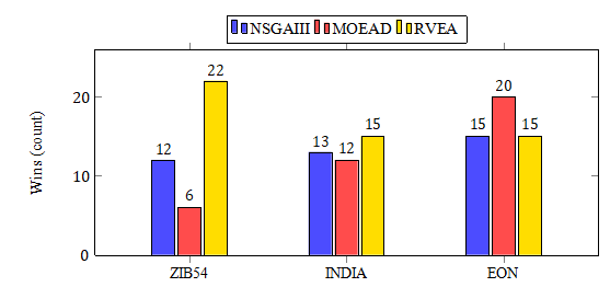
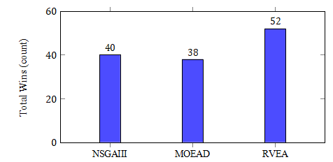
For example, inNET-zib54 with Traffic_2000, NSGA-III ran for 09:49:56, R-VEA for 09:18:53, and MOEA/D for 34:10:27—a ratio of approximately 3.7×.
Table 20: Wall-clock execution time per topology, traffic load, and algorithm (30 independent runs)
| Topology | Traffic | NSGA-III | R-VEA | MOEA/D |
|---|---|---|---|---|
| NET-EON-RT | Traffic_1500 | 01:34:54 | 01:26:26 | 05:01:52 |
| NET-EON-RT | Traffic_300 | 01:25:39 | 01:18:37 | 04:35:48 |
| NET-EON-RT | Traffic_340 | 01:25:10 | 01:17:00 | 04:36:52 |
| NET-EON-RT | Traffic_500 | 01:21:44 | 01:14:00 | 04:30:17 |
| NET-EON-RT | Traffic_980 | 01:26:28 | 01:16:02 | 04:43:55 |
| NET-INDIA35 | Traffic_1000 | 02:39:09 | 02:22:33 | 09:03:58 |
| NET-INDIA35 | Traffic_2000 | 02:53:21 | 02:38:50 | 09:47:48 |
| NET-INDIA35 | Traffic_400 | 02:38:29 | 02:24:02 | 09:08:40 |
| NET-INDIA35 | Traffic_600 | 02:31:04 | 02:21:17 | 08:31:29 |
| NET-zib54 | Traffic_1000 | 08:59:49 | 08:30:55 | 31:41:03 |
| NET-zib54 | Traffic_2000 | 09:49:56 | 09:18:53 | 34:10:27 |
| NET-zib54 | Traffic_3000 | 09:44:24 | 09:30:33 | 34:15:20 |
| NET-zib54 | Traffic_600 | 08:22:31 | 08:04:00 | 29:17:26 |
The higher execution cost of MOEA/D can be attributed to its de-composition strategy: in an 11-objective space, the algorithm must repeatedly evaluate Tchebycheff scalarizing functions and update subproblem neighborhoods for a large number of weight vectors, generating substantial overhead compared to the non-dominated sorting of NSGA-III or the angle-penalized distance of R-VEA. Notably, within each topology, the differences across traffic loads are minor (generally <20%), which confirms that network size—rather than request volume—is the primary driver of execution time.
8.6. Trade-offs Interpretation (QoS vs. OPEX/CAPEX)
One of the primary advantages of modeling VNF placement as a MaOP is the ability to expose the underlying conflicts between Quality of Service (QoS) metrics and Capital/Operational Expenditures (CAPEX/OPEX). In traditional single-objective approaches, minimizing costs often implicitly degrades service quality. How-ever, the Pareto fronts obtained by the MaOEAs allow network operators to quantify this degradation.For example, a solution that prioritizes OPEX reduction by consolidating VNFs into the minimum number of active servers (minimizing Energy Cost 𝑓1 and License Cost 𝑓10) inevitably forces traffic to traverse longer paths, thereby increasing Latency (𝑓3) and potentially decreasing the Network Effective Transfer Rate (𝑓16, QoS). Conversely, distributing VNFs close to the edge to maximize QoS requires provisioning more servers and software licenses, driving up OPEX.The extracted Pareto fronts consistently demonstrate that algorithms like R-VEA can provide solutions capable of maintaining high Throughput without disproportionately escalating Energy Costs or Distance, offering a balanced operational middle-ground for service providers across varying topologies such as EON-RT and zib54.
8.7. Statistical Validation
To statistically validate the performance among the MaOEAs, we employ the non-parametric Friedman test [67] alongside the Vargha-Delaney (𝐴12) effect size [68], and pairwise Wilcoxon rank-sum tests [69] over the Inverted Generational Distance (IGD) in-dicator. Because multiple pairwise comparisons are performed across various algorithms and scenarios, the Holm-Bonferroni procedure [70] is applied to adjust the 𝑝-values, thereby controlling the family-wise error rate (FWER) and preventing false positives (Type I errors). Table 21 presents a summary of the statistical tests across 30 independent runs per topology and traffic scenario. The results confirm that R-VEA is the dominant algorithm, outperforming MOEA/D and NSGA-III in the vast majority of cases. Specifically, against NSGA-III, the results show strong statistical significance (adjusted 𝑝 < 0.05) and large effect sizes (𝐴12 ≈ 0.99 − 1.0). When compared to MOEA/D, R-VEA maintains a clear advantage in terms of effect size (𝐴12 ≥ 0.77); however, in certain specific scenarios the adjusted 𝑝-value approaches 0.5, indicating a lack of statistical significance exclusively in those particular cases.
Table 21: Statistical validation (Friedman and Wilcoxon test, 𝑝 < 0.05) and Vargha-Delaney 𝐴12 for IGD
| Topology | Traffic | Best Algo | Compared Against | f12 |
|---|---|---|---|---|
| NET-EON-RT | 300, 500, 980, 1500 | R-VEA | MOEA/D, NSGA-III | 1.00 (+) |
| NET-INDIA35 | 400, 600, 1000, 2000 | R-VEA | MOEA/D, NSGA-III | 1.00 (+) |
| NET-zib54 | 600 | R-VEA | MOEA/D, NSGA-III | 0.86, 0.93 (+) |
| NET-zib54 | 1000, 2000 | R-VEA | MOEA/D, NSGA-III | 0.61 – 1.00 (+) |
| NET-zib54 | 3000 | MOEA/D | NSGA-III, R-VEA | 1.00 (+), 0.00 (=) |
The analysis of the statistical tests indicates a clear superiority of R-VEA in most configurations. The high Vargha-Delaney effect sizes (𝐴12 ranging from 0.77 to 1.0) combined with the extremely low 𝑝-values (𝑝 < 10−11 for the Friedman tests) provide strong empirical evidence that R-VEA consistently converges closer to the true Pareto front compared to NSGA-III and MOEA/D in the majority of evaluated scenarios.R-VEA’s dominant performance in this 11-objective space can be attributed to its reference vector guided approach and its Angle-Penalized Distance (APD) criterion. By dynamically adjusting its reference vectors based on the objective space geometry and balanc-ing convergence and diversity through the APD, R-VEA prevents the population from clustering in sub-optimal local regions—a frequent pathology in highly constrained combinatorial problems such as VNF placement. In contrast, NSGA-III’s reliance on Pareto dominance weakens as the number of objectives increases, and MOEA/D suffers from the computational overhead and rigidity of its scalarizing functions across so many dimensions.However, an interesting exception occurs in the NET-zib54 topology at the highest traffic load (Traffic_3000). Under this extreme congestion, the network’s resources are saturated, likely causing the true Pareto front to become highly disconnected, sparse, or severely distorted. In this specific boundary condition, the fixed reference vectors of R-VEA appear to struggle to adapt to the ir-regular front. Meanwhile, MOEA/D managed to find slightly better localized solutions through its weight-vector decomposition (𝐴12 = 1.0 against NSGA-III). This suggests that while R-VEA is generally the most robust and efficient algorithm for typical and moderately-high loads, decomposition-based strategies likeMOEA/D might offer slight advantages in ultra-congested, highly discontinuous boundary scenarios.8.8. Robustness AnalysisDue to the stochastic nature of evolutionary algorithms, analyzing their robustness across independent runs is critical. Figure 21 presents the distribution of the final Inverted Generational Distance (IGD) values achieved by each MaOEA across 30 independent executions under the highest traffic load for each topology. The boxplots reveal that NSGA-III and MOEA/D consistently attain lower IGD scores with very tight distributions (low variance), indi-cating highly stable and robust performance across different random initializations. Conversely, R-VEA exhibits a wider interquartile range and higher median IGD values, demonstrating greater sensitivity to the initial population and stochastic variations during the search process. This indicates that while R-VEA can find competitive individual solutions (as shown by other metrics), NSGA-III and MOEA/D provide more reliable and consistent overall approximations of the Pareto front.8.9. MANO Integration and Practical Edge DeploymentIn a practical NFV environment, the deployment of these solutions would be integrated into the NFV Management and Orchestration (MANO) framework. The MaOEA acts as an intelligent placement engine within the NFV Orchestrator (NFVO). Once the Pareto front is generated, a Multi-Criteria Decision Making (MCDM) method is required to select a single actionable solution based on the service provider’s dynamic priorities.
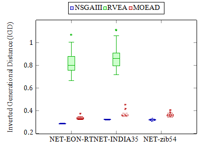
For instance, applying the TOPSIS (Technique for Order of Preference by Similarity to Ideal Solution) method to our resulting Pareto fronts with equal weights for all 11 retained objectives would yield a single solution characterized by a highly balanced trade-off. As an illustrative example, a representative placement configuration selected by TOPSIS could exhibit values of the order of: an Energy Cost around 9–10 units, a Delay Cost of approximately 17000 units, around 90–100 instantiated VNF instances, and a Throughput in the range of −30 to −25 units, achieving a TOPSIS composite score close to 0.86. This automated MCDM selection mechanism allows the MANO system to seamlessly bridge the gap between many-objective mathematical optimization and the physical instantiation of VNFs at the network edge.8.10. Limitations and Baseline ConsiderationsIt is important to acknowledge that this study focuses exclusively on comparing Many-Objective Evolutionary Algorithms (MaOEAs). A comparison against an exact baseline such as a Mixed Integer Linear Programming (MILP) solver or classical heuristic algorithms (e.g., Greedy First-Fit) was not included in our experimental setup. The VNF Placement problem is inherently NP-Hard, and as widely demonstrated in the literature, exact MILP models scale exponentially with both network size and constraint complexity. Consequently, solving a MILP formulation that simultaneously incorporates 11 conflicting objectives is computationally intractable for the large topologies evaluated in our study (such as NET-INDIA35 and NET-zib54). Furthermore, adapting traditional Greedy heuristics to navigate an 11-dimensional objective space without introducing significant scalarization bias is highly complex and remains outside the scope of this work. Therefore, our reliance on MaOEAs is fundamentally motivated by the critical need to discover acceptable, near-optimal multi-objective trade-offs within practical computational timeframes, specifically in large-scale scenarios where exact methods are structurally incapable of scaling.
9. Conclusions and Future Work
Based on the key contributions of this work, which include the correlation analysis within the state of the art and the performance comparison of evolutionary algorithms (NSGA-III, R-VEA, and MOEA/D) for optimizing VNF placement to guarantee QoS and reduce CAPEX and OPEX, the following conclusions can be drawn:
- Correlation Analysis: The first major contribution of this work consisted of performing a correlation analysis of the state of the art, which is a crucial step to simplify and reduce the complexity of the optimization By identifying the relationships among the objectives, the number of objectives to be optimized can be reduced, thereby facilitating the search for more effective solutions. This can simplify the search process, render the problem more manageable, and lead to faster convergence of the optimization algorithms as well as the obtainment of more practical and efficient solutions.
- Algorithm Comparison: The second contribution focuses on comparing the performance of evolutionary algorithms under rigorous statistical Through non-parametric Friedman testing and pairwise Wilcoxon tests (adjusted 𝑝 < 0.05 via Holm-Bonferroni) and Vargha-Delaney effect sizes (𝐴12 ≥ 0.86), the results indicate that R-VEA consistently demonstrates superior performance across most topologies and load scenarios. This robustness is attributed to its Angle-Penalized Distance (APD) metric, which adeptly balances convergence and diversity in highly dimensional Pareto fronts. This performance consistency suggests that R-VEA is a reliable and effective option for addressing the VNF placement problem with multiple objectives, except in highly saturated network edge cases where MOEA/D occasionally exhibited resilience due to Pareto front distortion.
- Practical Implications for Network Operators: Finally, the formulated many-objective optimization framework of-fers tangible benefits for telecommunication operators mi-grating to NFV By demonstrating that algo-rithms like R-VEA can successfully balance conflicting operational dimensions—such as minimizing energy consumption (OPEX) and server installations (CAPEX) while adhering to SLA delay bounds (QoS)—network administrators are provided with a robust decision-support tool. This capabil-ity enables operators to select deployment configurations tailored to specific business policies, effectively reducing infrastructure footprint without sacrificing user experience.
In summary, this work has made significant contributions by addressing the VNF placement optimization problem in networks. The simplification through correlation analysis and the effective selection of the R-VEA algorithm have led to promising results in terms of generating high-performance solutions on the Pareto front. These conclusions support the utility and applicability of this approach to improve network resource management concerning QoS, CAPEX, and OPEX. In addition to the current contributions, several research areas for future work are proposed, which could expand and enrich the field:
- Dynamic adaptability of the algorithms: Extending the VNFplacement problem from a static scenario to a dynamic one, where the topology, traffic load, and service chains vary over time. In this context, it is relevant to study adaptive variants of R-VEA, MOEA/D, and NSGA-III that incorpo-rate memory mechanisms, change detection, and population reheating in order to maintain the quality of the Pareto front in the face of events such as link failures, traffic spikes, or the deployment of new services.
- Impact ofobjective reduction on decision-making: Con-ducting a systematic study comparing the solutions obtained when utilizing all objective functions versus the case where only the subset reduced via Pearson correlations is The analysis should evaluate how VNF placement, link uti-lization, node consolidation, and QoS levels change, as well as the shape of the approximated Pareto front. A key aspect is to quantify how much is lost (or gained) in terms of solution quality, robustness, and variety of alternatives for the operator when working with a reduced but computationally and interpretatively lighter model.
- Comparison and improvement of objective reduction schemes: Delving into the comparison between objective function selection based on Pearson correlations and other dimensionality reduction approaches (e.g., PCA, mutual in-formation analysis, or objective clustering). An interesting future work is to systematically analyze how each reduction scheme impacts the convergence, Pareto front diversity, and computational cost of many-objective evolutionary algorithms applied to the VNF placement problem.
- Evaluation inlarge-scale scenarios and with real traces: Replicating and extending the conducted experiments to larger and more heterogeneous topologies (e.g., operator WAN networks, 5G/edge scenarios, or multi-domain net-works), as well as utilizing real traffic traces and demand patterns. This would allow validating the robustness of the algorithms and the reduced set of objective functions in operational contexts closer to production deployments.
- Hybridizationwith machine learning techniques: Invest-gating the integration of machine learning models to assist the evolutionary process, whether through traffic pattern predic-tion, construction of surrogate models to estimate expensive objective functions, or dynamic adjustment of evolutionary This hybridization could reduce execution times and improve the system’s response in online scenarios.
- Thoroughbaseline comparison: Conducting a comprehen-sive comparison against exact methods (e.g., Mixed Integer Linear Programming formulations) or specialized state-of-the-art single-objective While a full MILP evalua-tion is computationally intractable at the scale of our current experiments due to the combination of 11 objectives and large network instances, establishing these baselines on smaller-scale scenarios or using simplified models constitutes an important direction to quantify the optimality gap and fur-ther validate the relative effectiveness of the many-objective evolutionary approach.
These lines of future work seek to delve deeper into the treatment of the dynamic nature of the VNF placement problem, improve objective reduction strategies, and bring evolutionary proposals closer to realistic operation scenarios, thereby strengthening the practical applicability of many-objective optimization in NFV-based networks.
- ETSI Industry Specification Group for Network Functions Virtualisation, “Network Functions Virtualisation: An Introduction, Benefits, Enablers, Challenges and Call for Action,” Technical report, ETSI, 2012.
- J. Billingsley, K. Li, W. Miao, G. Min, N. Georgalas, “A Formal Model for Multi-objective Optimisation of Network Function Virtualisation Placement,” in International Conference on Evolutionary Multi-Criterion Optimization, 529–540, Springer, 2019, doi:10.1007/978-3-030-12598-1_42
- J. Martins, M. Ahmed, C. Raiciu, V. Olteanu, M. Honda, R. Bifulco, F. Huici, “ClickOS and the Art of Network Function Virtualization,” in Proceedings of the 11th USENIX Symposium on Networked Systems Design and Implementation (NSDI 14), 459–473, 2014.
- B. Yi, X. Wang, K. Li, M. Huang, et al., “A comprehensive survey of network function virtualization,” Computer Networks, 133, 212–262, 2018, doi:10.1016/j.comnet.2018.01.021
- M. F. Bari, S. R. Chowdhury, R. Ahmed, R. Boutaba, “On orchestrating virtual network functions,” in 2015 11th International Conference on Network and Service Management (CNSM), 50–56, IEEE, 2015, doi:10.1109/cnsm.2015.7367338
- F. Bari, S. R. Chowdhury, R. Ahmed, R. Boutaba, O. C. M. B. Duarte, “Orchestrating virtualized network functions,” IEEE Transactions on Network and Service Management, 13(4), 725–739, 2016, doi:10.1109/tnsm.2016.2569020
- C. A. C. Coello, “Computación Evolutiva,” Incomplete source details in the original BibTeX file.
- B. Addis, D. Belabed, M. Bouet, S. Secci, “Virtual network functions placement and routing optimization,” in 2015 IEEE 4th International Conference on Cloud Networking (CloudNet), 171–177, IEEE, 2015, doi:10.1109/cloudnet.2015.7335301
- M. Gao, B. Addis, M. Bouet, S. Secci, “Optimal orchestration of virtual network functions,” Computer Networks, 142, 108–127, 2018, doi:10.1016/j.comnet.2018.06.006
- S. Lange, A. Grigorjew, T. Zinner, P. Tran-Gia, M. Jarschel, “A multi-objective heuristic for the optimization of virtual network function chain placement,” in 2017 29th International Teletraffic Congress (ITC 29), volume 1, 152–160, IEEE, 2017, doi:10.23919/itc.2017.8064351
- K. Deb, A. Pratap, S. Agarwal, T. Meyarivan, “A fast and elitist multiobjective genetic algorithm: NSGA-II,” IEEE transactions on evolutionary computation, 6(2), 182–197, 2002, doi:10.1109/4235.996017
- C. Von Lücken, B. Barán, C. Brizuela, “A survey on multi-objective evolutionary algorithms for many-objective problems,” Computational optimization and applications, 58(3), 707–756, 2014, doi:10.1007/s10589-014-9644-1
- S. Chand, M. Wagner, “Evolutionary Many-Objective Optimization: A Quick-Start Guide,” Surveys in Operations Research and Management Science, 20(2), 35–42, 2015, doi:10.1016/j.sorms.2015.08.001
- D. Kreutz, F. M. V. Ramos, P. E. Verissimo, C. E. Rothenberg, S. Azodolmolky, S. Uhlig, “Software-Defined Networking: A Comprehensive Survey,” IEEE Communications Surveys & Tutorials, 17(1), 14–76, 2015, doi:10.1109/SURV.2014.032014.00182
- P. Barham, B. Dragovic, K. Fraser, S. Hand, T. Harris, A. Ho, R. Neugebauer, I. Pratt, A. Warfield, “Xen and the art of virtualization,” in ACM SIGOPS Operating Systems Review, volume 37, 164–177, 2003, doi:10.1145/1165389.945462
- A. Tomassilli, F. Giroire, N. Huin, S. Pérennes, “Provably efficient algorithms for placement of service function chains with ordering constraints,” in IEEE INFOCOM 2018-IEEE Conference on Computer Communications, 774–782, IEEE, 2018, doi:10.1109/infocom.2018.8486275
- O. Soualah, M. Mechtri, C. Ghribi, D. Zeghlache, “Online and batch algorithms for VNFs placement and chaining,” Computer Networks, 158, 98–113, 2019, doi:10.1016/j.comnet.2019.01.041
- O. Soualah, M. Mechtri, C. Ghribi, D. Zeghlache, “Energy efficient algorithm for VNF placement and chaining,” in 2017 17th IEEE/ACM International Symposium on Cluster, Cloud and Grid Computing (CCGRID), 579–588, IEEE, 2017, doi:10.1109/ccgrid.2017.84
- M. A. Raayatpanah, T.Weise, “Virtual network function placement for service function chaining with minimum energy consumption,” in 2018 IEEE International Conference on Computer and Communication Engineering Technology (CCET), 198–202, IEEE, 2018, doi:10.1109/ccet.2018.8542223
- D. Amaya, Y. Sumi, S. Homma, T. Okugawa, T. Tachibana, “VNF placement with optimization problem based on data throughput for service chaining,” in 2018 IEEE 7th International Conference on Cloud Networking (CloudNet), 1–3, IEEE, 2018, doi:10.1109/cloudnet.2018.8549543
- A. Alleg, T. Ahmed, M. Mosbah, R. Riggio, R. Boutaba, “Delay-aware VNF placement and chaining based on a flexible resource allocation approach,” in 2017 13th International Conference on Network and Service Management (CNSM), 1–7, ieee, 2017, doi:10.23919/cnsm.2017.8255993
- M. Savi, M. Tornatore, G. Verticale, “Impact of processing-resource sharing on the placement of chained virtual network functions,” IEEE Transactions on Cloud Computing, 2019, doi:10.1109/tcc.2019.2914387
- A. Gupta, M. F. Habib, P. Chowdhury, M. Tornatore, B. Mukherjee, “Joint virtual network function placement and routing of traffic in operator networks,” UC Davis, Davis, CA, USA, Tech. Rep, 2015.
- O. Soualah, M. Mechtri, C. Ghribi, D. Zeghlache, “A green VNFs placement and chaining algorithm,” in NOMS 2018-2018 IEEE/IFIP Network Operations and Management Symposium, 1–5, IEEE, 2018, doi:10.1109/noms.2018.8406183
- M. C. Luizelli, L. R. Bays, L. S. Buriol, M. P. Barcellos, L. P. Gaspary, “Piecing together the NFV provisioning puzzle: Efficient placement and chaining of virtual network functions,” in 2015 IFIP/IEEE International Symposium on Integrated Network Management (IM), 98–106, IEEE, 2015, doi:10.1109/inm.2015.7140281
- Y. Sang, B. Ji, G. R. Gupta, X. Du, L. Ye, “Provably efficient algorithms for joint placement and allocation of virtual network functions,” in IEEE INFOCOM 2017-IEEE Conference on Computer Communications, 1–9, IEEE, 2017, doi:10.1109/infocom.2017.8057036
- M. C. Luizelli, W. L. da Costa Cordeiro, L. S. Buriol, L. P. Gaspary, “A fix-and-optimize approach for efficient and large scale virtual network function placement and chaining,” Computer Communications, 102, 67–77, 2017, doi:10.1016/j.comcom.2016.11.002
- H. Xing, X. Zhou, X. Wang, S. Luo, P. Dai, K. Li, H. Yang, “An integer encoding grey wolf optimizer for virtual network function placement,” Applied Soft Computing, 76, 575–594, 2019, doi:10.1016/j.asoc.2018.12.037
- R. Cziva, C. Anagnostopoulos, D. P. Pezaros, “Dynamic, latencyoptimal vNF placement at the network edge,” in Ieee infocom 2018-ieee conference on computer communications, 693–701, IEEE, 2018, doi:10.1109/infocom.2018.8486021
- D. B. Oljira, K.-J. Grinnemo, J. Taheri, A. Brunstrom, “A model for QoS-aware VNF placement and provisioning,” in 2017 IEEE Conference on Network Function Virtualization and Software Defined Networks (NFV-SDN), 1–7, IEEE, 2017, doi:10.1109/nfv-sdn.2017.8169829
- Z. Allybokus, N. Perrot, J. Leguay, L. Maggi, E. Gourdin, “Virtual function placement for service chaining with partial orders and anti-affinity rules,” Networks, 71(2), 97–106, 2018, doi:10.1002/net.21768
- M. Ghaznavi, A. Khan, N. Shahriar, K. Alsubhi, R. Ahmed, R. Boutaba, “Elastic virtual network function placement,” in 2015 IEEE 4th International Conference on Cloud Networking (CloudNet), 255–260, IEEE, 2015, doi:10.1109/cloudnet.2015.7335318
- C. Pham, N. H. Tran, S. Ren, W. Saad, C. S. Hong, “Traffic-aware and energy-efficient vnf placement for service chaining: Joint sampling and matching approach,” IEEE Transactions on Services Computing, 2017, doi:10.1109/tsc.2017.2671867
- O. A. Wahab, N. Kara, C. Edstrom, Y. Lemieux, “MAPLE: A Machine Learning Approach for Efficient Placement and Adjustment of Virtual Network Functions,” Journal of Network and Computer Applications, 142, 37–50, 2019, doi:10.1016/j.jnca.2019.06.003
- D. Qi, S. Shen, G. Wang, “Towards an efficient VNF placement in network function virtualization,” Computer Communications, 138, 81–89, 2019, doi:10.1016/j.comcom.2019.03.005
- H. Moens, F. De Turck, “VNF-P: A model for efficient placement of virtualized network functions,” in 10th International Conference on Network and Service Management (CNSM) and Workshop, 418–423, IEEE, 2014, doi:10.1109/cnsm.2014.7014205
- P. Vizarreta, M. Condoluci, C. M. Machuca, T. Mahmoodi,W. Kellerer, “QoSdriven function placement reducing expenditures in NFV deployments,” in 2017 IEEE International Conference on Communications (ICC), 1–7, IEEE, 2017, doi:10.1109/icc.2017.7996513
- S. Mehraghdam, M. Keller, H. Karl, “Specifying and placing chains of virtual network functions,” in 2014 IEEE 3rd International Conference on Cloud Networking (CloudNet), 7–13, IEEE, 2014, doi:10.1109/cloudnet.2014.6968961
- S. Ahvar, H. P. Phyu, S. M. Buddhacharya, E. Ahvar, N. Crespi, R. Glitho, “CCVP: Cost-efficient centrality-based VNF placement and chaining algorithm for network service provisioning,” in 2017 IEEE Conference on Network Softwarization (NetSoft), 1–9, IEEE, 2017, doi:10.1109/netsoft.2017.8004104
- X. Song, X. Zhang, S. Yu, S. Jiao, Z. Xu, “Resource-efficient virtual network function placement in operator networks,” in GLOBECOM 2017-2017 IEEE Global Communications Conference, 1–7, IEEE, 2017, doi:10.1109/glocom.2017.8254492
- T.-H. Nguyen, J. Lee, M. Yoo, “A Practical Model for Optimal Placement of Virtual Network Functions,” in 2019 International Conference on Information Networking (ICOIN), 239–241, IEEE, 2019, doi:10.1109/icoin.2019.8717979
- R. Cohen, L. Lewin-Eytan, J. S. Naor, D. Raz, “Near optimal placement of virtual network functions,” in 2015 IEEE Conference on Computer Communications (INFOCOM), 1346–1354, IEEE, 2015, doi:10.1109/infocom.2015.7218511
- S. Tavakoli-Someh, M. H. Rezvani, “Multi-objective virtual network function placement using NSGA-II meta-heuristic approach,” The Journal of Supercomputing, 1–37, 2019, doi:10.1007/s11227-019-02849-y
- S. Khebbache, M. Hadji, D. Zeghlache, “A Multi-Objective Non-Dominated Sorting Genetic Algorithm for VNF Chains Placement,” in 2018 15th IEEE Annual Consumer Communications & Networking Conference (CCNC), 1–4, IEEE, 2018, doi:10.1109/CCNC.2018.8319250
- C. A. C. Coello, G. B. Lamont, D. A. Van Veldhuizen, et al., Evolutionary algorithms for solving multi-objective problems, volume 5, Springer, 2007, doi:10.1007/978-1-4757-5184-0
- K. Deb, “Multi-objective optimisation using evolutionary algorithms: an introduction,” in Multi-objective evolutionary optimisation for product design and manufacturing, 3–34, Springer, 2011, doi:10.1007/978-0-85729-652-8_1
- K. Deb, Multi-Objective Optimization Using Evolutionary Algorithms, John Wiley & Sons, 2001.
- M. Farina, P. Amato, “On the Optimal Solution Definition for Many-Criteria Optimization Problems,” in 2002 Annual Meeting of the North American Fuzzy Information Processing Society Proceedings, NAFIPS-FLINT 2002, 233–238, IEEE, 2002, doi:10.1109/NAFIPS.2002.1018061
- S. Khebbache, M. Hadji, D. Zeghlache, “Scalable and cost-efficient algorithms for VNF chaining and placement problem,” in 2017 20th conference on innovations in clouds, internet and networks (ICIN), 92–99, IEEE, 2017, doi:10.1109/icin.2017.7899395
- E. Zitzler, L. Thiele, M. Laumanns, C. Fonseca, V. da Fonseca, “Performance assessment of multiobjective optimizers: an analysis and review,” IEEE Transactions on Evolutionary Computation, 7(2), 117–132, 2003, doi:10.1109/TEVC.2003.810758
- K. C. Tan, T. H. Lee, E. F. Khor, “Evolutionary Algorithms for Multi-Objective Optimization: Performance Assessments and Comparisons,” Artificial Intelligence Review, 17(4), 251–290, 2002, doi:10.1023/A:1015516501242
- D. Hadka, “MOEA Framework: A Free and Open Source Java Framework for Multiobjective Optimization,” 2025, version 5.1 [Computer software].
- K. Bringmann, T. Friedrich, “Computing the hypervolume indicator: exact algorithms, approximations, and lower bounds,” Artificial Intelligence, 205, 100–122, 2013.
- L. While, L. Bradstreet, L. Barone, “A fast way of calculating exact hypervolumes,” IEEE Transactions on Evolutionary Computation, 16(1), 86–95, 2012, doi:10.1109/tevc.2010.2077298
- N. Beume, C. M. Fonseca, M. Lopez-Ibanez, L. Paquete, J. Vahrenhold, “The complexity of computing the hypervolume indicator,” IEEE Transactions on Evolutionary Computation, 13(5), 1075–1082, 2009, doi:10.1109/tevc.2009.2015575
- J. Miao, L. Niu, “A Survey on Feature Selection,” Procedia Computer Science, 91, 919–926, 2016, doi:10.1016/j.procs.2016.07.111
- N. Honest, K. Kotecha, “A survey on feature selection techniques,” International Journal of Computer Applications, 975(8887), 1–6, 2020.
- B. G. Bathula, J. M. Elmirghani, “Constraint-based anycasting over optical burst switched networks,” Journal of Optical Communications and Networking, 1(2), A35–A43, 2009, doi:10.1364/jocn.1.000a35
- M. Yang, K. Guo, Y. Zhang, Y. Ji, “Routing, modulation level, spectrum and transceiver assignment in elastic optical networks,” IEICE Transactions on Communications, 101(5), 1197–1209, 2018, doi:10.1587/transcom.2017ebp3309
- M. K. Awad, Y. Rafique, S. Alhadlaq, D. Hassoun, A. Alabdulhadi, S. Thani, “A greedy power-aware routing algorithm for softwaredefined networks,” in 2016 IEEE International Symposium on Signal Processing and Information Technology (ISSPIT), 268–273, IEEE, 2016, doi:10.1109/isspit.2016.7886047
- R. Cheng, Y. Jin, M. Olhofer, B. Sendhoff, “A Reference Vector Guided Evolutionary Algorithm for Many-Objective Optimization,” IEEE Transactions on Evolutionary Computation, 20(5), 773–791, 2016, doi:10.1109/TEVC.2016.2519378
- Q. Zhang, H. Li, “MOEA/D: A Multiobjective Evolutionary Algorithm Based on Decomposition,” IEEE Transactions on Evolutionary Computation, 11(6), 712–731, 2007, doi:10.1109/TEVC.2007.892759
- K. Deb, H. Jain, “An Evolutionary Many-Objective Optimization Algorithm Using Reference-Point-Based Nondominated Sorting Approach, Part I: Solving Problems with Box Constraints,” IEEE Transactions on Evolutionary Computation, 18(4), 577–601, 2014, doi:10.1109/TEVC.2013.2281535
- K. Deb, R. B. Agrawal, “Simulated binary crossover for continuous search space,” Complex Systems, 9(2), 115–148, 1995.
- R. Storn, K. Price, “Differential evolution–a simple and efficient heuristic for global optimization over continuous spaces,” Journal of Global Optimization, 11(4), 341–359, 1997, doi:10.1023/a:1008202821328
- Zuse Institute Berlin, “ZIB54 Network Topology,” Benchmark network instance, network with 54 nodes.
- M. Friedman, “The use of ranks to avoid the assumption of normality implicit in the analysis of variance,” Journal of the american statistical association, 32(200), 675–701, 1937, doi:10.1080/01621459.1937.10503522
- A. Vargha, H. D. Delaney, “A critique and improvement of the CL common language effect size statistics of McGraw and Wong,” Journal of Educational and Behavioral Statistics, 25(2), 101–132, 2000, doi:10.3102/10769986025002101
- F. Wilcoxon, “Individual comparisons by ranking methods,” Biometrics bulletin, 1(6), 80–83, 1945, doi:10.2307/3001968
- S. Holm, “A simple sequentially rejective multiple test procedure,” Scandinavian journal of statistics, 65–70, 1979, doi:10.2307/4615733